Living in Philadelphia allows me to travel to New York City easily during my casual time. Observing this busy yet vibrant city is an unforgettable experience.
Alaska, USA, 2021
After the end of Spring 2021 semester, I went on a trip to Alaska with my friends Zhihao Ruan and Kun Huang. It is a wonderful place to travel if you love snow mountains and glaciers. We enjoyed it a lot.
Quadrotors Minimum Snap Trajectory Generation and Control for Obstacle Avoidance
This is the open-ended final project I conducted for the course ESE 650 “Learning in Robotics” at the University of Pennsylvania. My collaborator on this project is Zhihao Ruan.
For the demonstration of results for this project, please see the following video:
More technical information is introduced in this report:
F1Tenth Autonomous Racing Cars Independent Study Project - Multi-Vehicle Coordination for Overtaking Maneuvers
During the Spring 2021 semester, I joined the F1Tenth team at Penn to conduct an interest project on multi-vehicle coordination. My collaborator on this project is Wesley Yee.
For the details and results of this project, please refer to the following report:
F1Tenth Autonomous Racing Cars - Lab 7 (RRT and RRT*)
During the Spring 2021 semester, I joined the F1Tenth team at Penn to conduct an interest project on multi-vehicle coordination. Lab 7 of the “F1Tenth” course is focused on RRT and RRT* that could be fundamental to my project, so I have completed it and will demonstrate below.
Overview
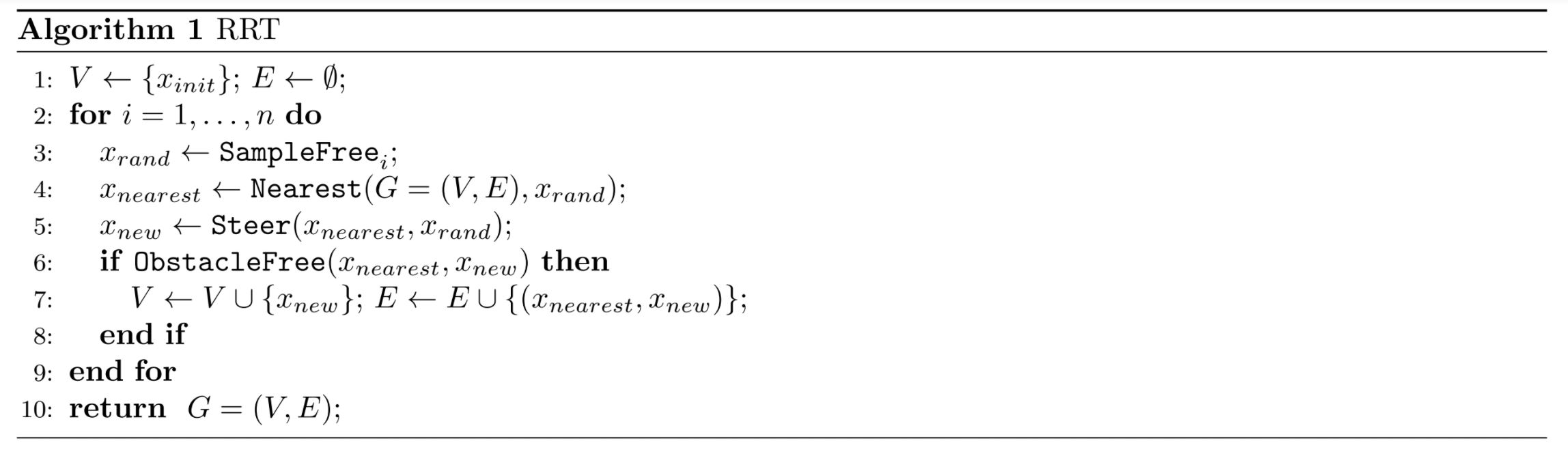
This post contains my results for Lab 7, where the RRT and RRT* algorithm for path planning is implemented for the race car so that it can generate a set of desired waypoints to the goal. The Pure Pursuit algorithm in lab 6 is used for tracking the corresponding generated waypoints. They together allows the car to complete a loop of the Levine Hall smoothly. See the video below for a demonstration of the RRT algorithm:
Demonstration of RRT
In the video, the red point is the goal point manually set according to the location of the car in the map; the blue points are the sampled points from the RRT algorithm; the green trajectory is the path found by the RRT algorithm; and the green point is the waypoint the car currently is following (so that the car can follow the green trajectory). Improvements were made that resulted in an implementation of the RRT* algorithm, which will be demonstrated later in this post.
Procedure
The first step of the RRT algorithm is to define the goal point (the red point in the above figure). I defined them according to the current location of the car in the map. The algorithm then iteratively samples random point in a designated region (also defined according to the current location of the car in the map). A tree is maintained through this process and each iteration steers a node of the tree (the closest node) to the direction of the sampled point. The process is terminated when either the goal point is reached by the tree or the desired maximum number of iterations is reached. If the goal point is reached, we can then trace back the tree to find the desired trajectory. A pseudo code of the algorithm is presented below:
 RRT pseudo code.
A clear disadvantage of this algorithm is its suboptimality. The generated paths are non-smooth and hard to follow by the race cars. See the figure below,
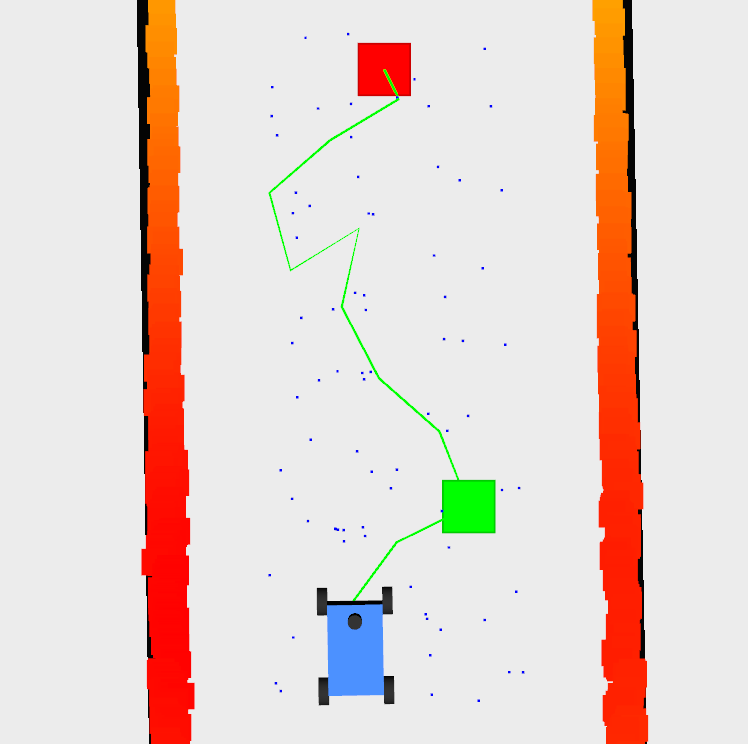 Non-smooth path generated by RRT.
A solution to this is to use the RRT* algorithm, which is an algorithm built on RRT, but rewiring the tree while adding new nodes to it, a pseudo code of the algorithm is presented below:
](/2021/02/20/f1tenth-lab-7/RRTstar_CODE.JPG) [RRT* pseudo code.](https://arxiv.org/pdf/1105.1186.pdf)
[RRT* pseudo code.](https://arxiv.org/pdf/1105.1186.pdf)
The result of the RRT* algorithm is shown below for comparison to the result of RRT, a video demonstration is also shown in the next section:
 Smoooth path generated by RRT*.
More technical details can be found in the below prompt document and this paper:
My source codes for this lab can be found on github through this link.
Demonstration of RRT*
The generated path is obviously smoother with the RRT*.
Reference
The lecture video can be found below:
F1Tenth Autonomous Racing Cars - Lab 6 (Pure Pursuit)
During the Spring 2021 semester, I joined the F1Tenth team at Penn to conduct an interest project on multi-vehicle coordination. To get prepared for the project, I self-learned and completed Lab 1, 2, 3, 4, and 6 of the “F1Tenth” course.
Overview
This post contains my results for Lab 6, where the Pure Pursuit algorithm for path tracking is implemented for the race car so that it can follow the designated waypoints, completing a loop of the Levine Hall smoothly. See the video below for a cool demonstration of the Pure Pursuit algorithm:
Demonstration
Of course the above is the situation where I pushed the algorithm to its limit, so that the vehicle starts drifting in order to complete the loop as fast as possible. The vehicle can track the waypoints better if we drive slower as in lab3 and lab4, as shown in video below:
Procedure
I first generated the waypoints by localizing the vehicle in the desired map (Levine Hall) using a Particle Filter and recording the locations with a Waypoint Logger. Notice that the Particle Filter implementation provided in the link requires Python 2 environment to build. However, from my experience, the node will run successfully even in a Python 3 environment as long as the codes are modified to their “Python 3” version (such as “print”), a modified version can be found here.
Another note is that a predefined map is required for generating the waypoints. In my case, I could not get in touch with a real car due to the COVID-19 pandemic, so I chose to use a provided map for the simulation. However, it is possible to generate a map ourselves with SLAM. Check out Google Cartographer for more information.
With the waypoints, the Pure Pursuit algorithm can be summarized in the following steps:
- Localize the vehicle with some localization methods, for example, particle filter. This allows the vehicle to identify its nearby waypoints and their relative position in future steps.
- Choose the next appropriate waypoint according to some lookahead distance L. In my code implementation, I chose the closest waypoint that is in the “half plane” that the vehicle is oriented and has a distance greater than L to the vehicle. Note that the lookahead distance L can be tuned to achieve desired performance.
- Calculate the required steering angle to reach the desired point. This calculation is non-trivial due to the non-holonomic nature of cars. See the picture below, due to the velocity and heading of the vehicle, we would not reach the goal point smoothly (possibly with large overshoot) if we just set the steering angle to the exact direction of the goal point. Therefore, we want to find an arc between the current position and the goal point for smooth movement of the vehicle. Since there will be infinitely many arcs possible to this purpose, we define our desired arc as the one whose center of radius lies on the y-axis of the vehicle’s coordinate frame. The curvature of the arc can then be calculated with the equation in the picture below. Finally, the required steering angle was set to be proportional to this curvature, subject to a scaling factor KP, just as a P controller where the gain KP can be tuned to obatin desired performance.
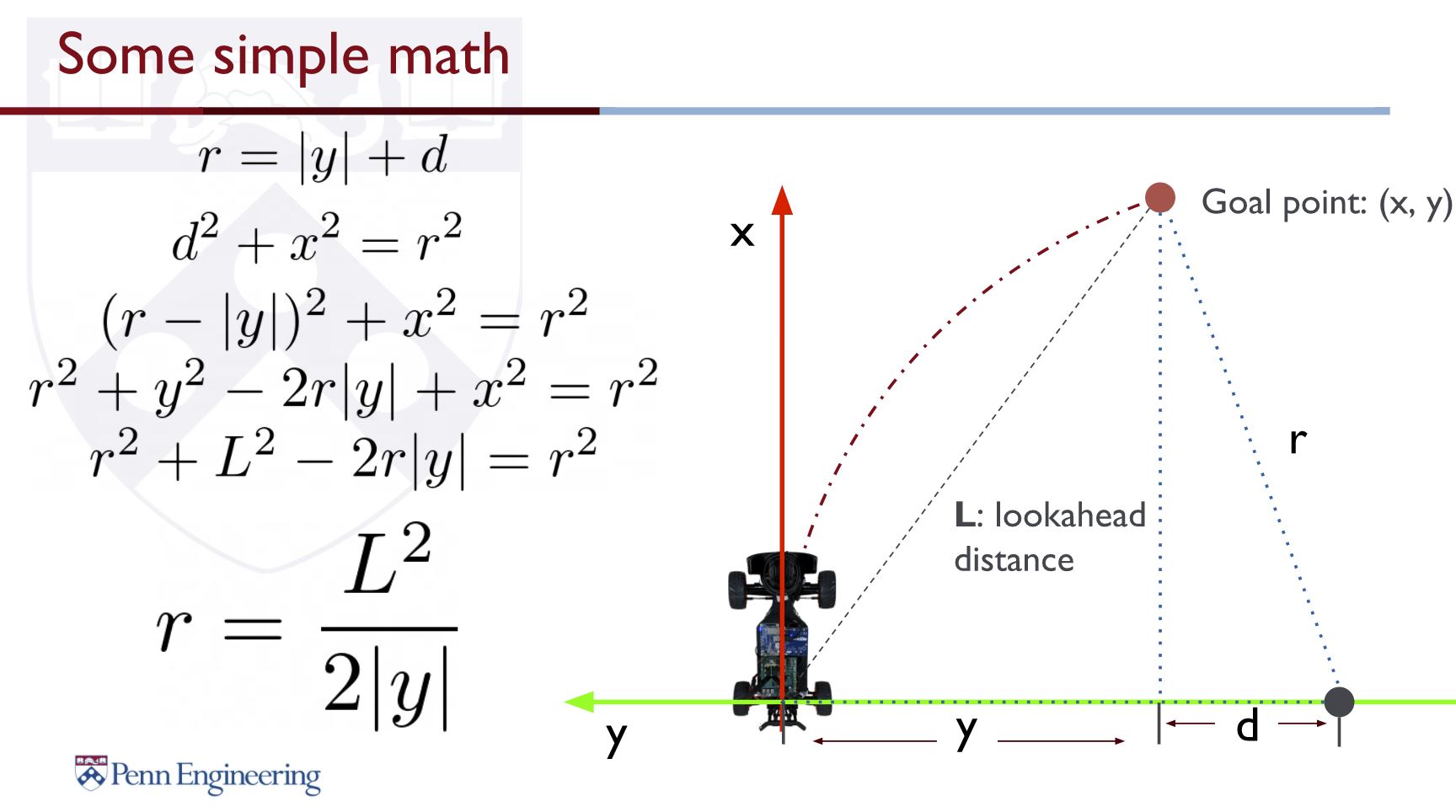 Steering angle calculation to reach a goal point.
- Publish the desired steering angle and speed to the vehicle.
More technical details can be found in the below prompt document:
My source codes for this lab can be found on github through this link.
Reference
The lecture video can be found below:
F1Tenth Autonomous Racing Cars - Lab 4 (Reactive Planner "Follow the Gap")
During the Spring 2021 semester, I joined the F1Tenth team at Penn to conduct an interest project on multi-vehicle coordination. To get prepared for the project, I self-learned and completed Lab 1, 2, 3, 4, and 6 of the “F1Tenth” course.
Overview
This post contains my results for Lab 4, where a reactive planning method for obstable avoidance “Follow the Gap” is implemented for the race car so that it can avoid obstacles and complete a loop of the Levine Hall smoothly. See the video below for a demonstration of the reactive planner:
Demonstration
Procedure
The big picture of the algorithm is shown below:
 The general steps of the "Follow the Gap" algorithm.
My customized implementation of the algorithm can be summarized in the following steps:
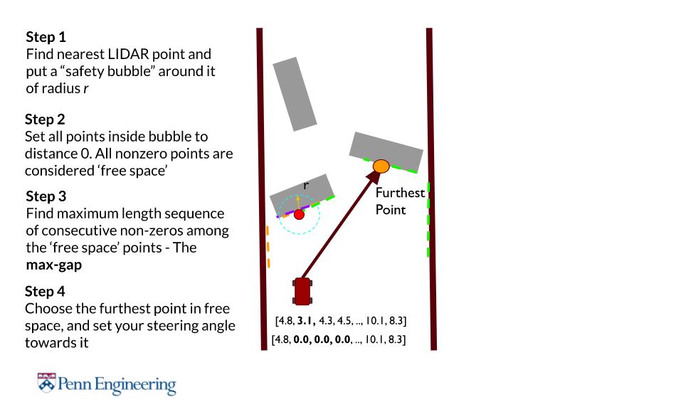
- Obtain laser scans and preprocess them: Since the laser scan data will be accompanied with noises and potential “nan” or “inf” values, I first clip the laser scan data into a range of [0, range_max] (range_max is provided by the lidar message itself, indicating the maximum valid laser scan data). Then I used a sliding window of size 5 to obtain average values of the laser scan data, which could help with eliminating the noises.
- Find the closest point in the lidar scan data: In this step I use the preprocessed lidar scan data to find the closest point in the vehicle’s front of view (between -70 and 70 degrees).
- Draw a safety “bubble” around this closest point and set all points inside this “bubble” to 0. All other non-zero points are now considered “gaps” or “free space”.
- Find the max length “gap”, in other words, the largest number of consecutive non-zero elements in the processed lidar scan data array.
- Find the best goal point in this gap. This is defined to be the furthest point away in the gap. In the case of multiple points sharing the same distance, the one that is at the smallest absolute angle to the vehicle’s frame will be chosen as the goal point.
- Actuate the car to move towards this goal point.
More technical details can be found in the below prompt document:
My source codes for this lab can be found on github through this link.
Reference
The lecture video can be found below:
F1Tenth Autonomous Racing Cars - Lab 3 (Wall Following with PID Controller)
During the Spring 2021 semester, I joined the F1Tenth team at Penn to conduct an interest project on multi-vehicle coordination. To get prepared for the project, I self-learned and completed Lab 1, 2, 3, 4, and 6 of the “F1Tenth” course.
Overview
This post contains my results for Lab 3, where a PID controller for wall following is implemented for the race car so that it can follow the inner walls of the Levine Hall and complete a loop smoothly. See the video below for a demonstration of the wall follower:
Demonstration
Procedure
I calculated the vehicle’s distance to the wall from its 2d-lidar scan information, this is done by using the 2d-lidar scan data from two directions as shown below:
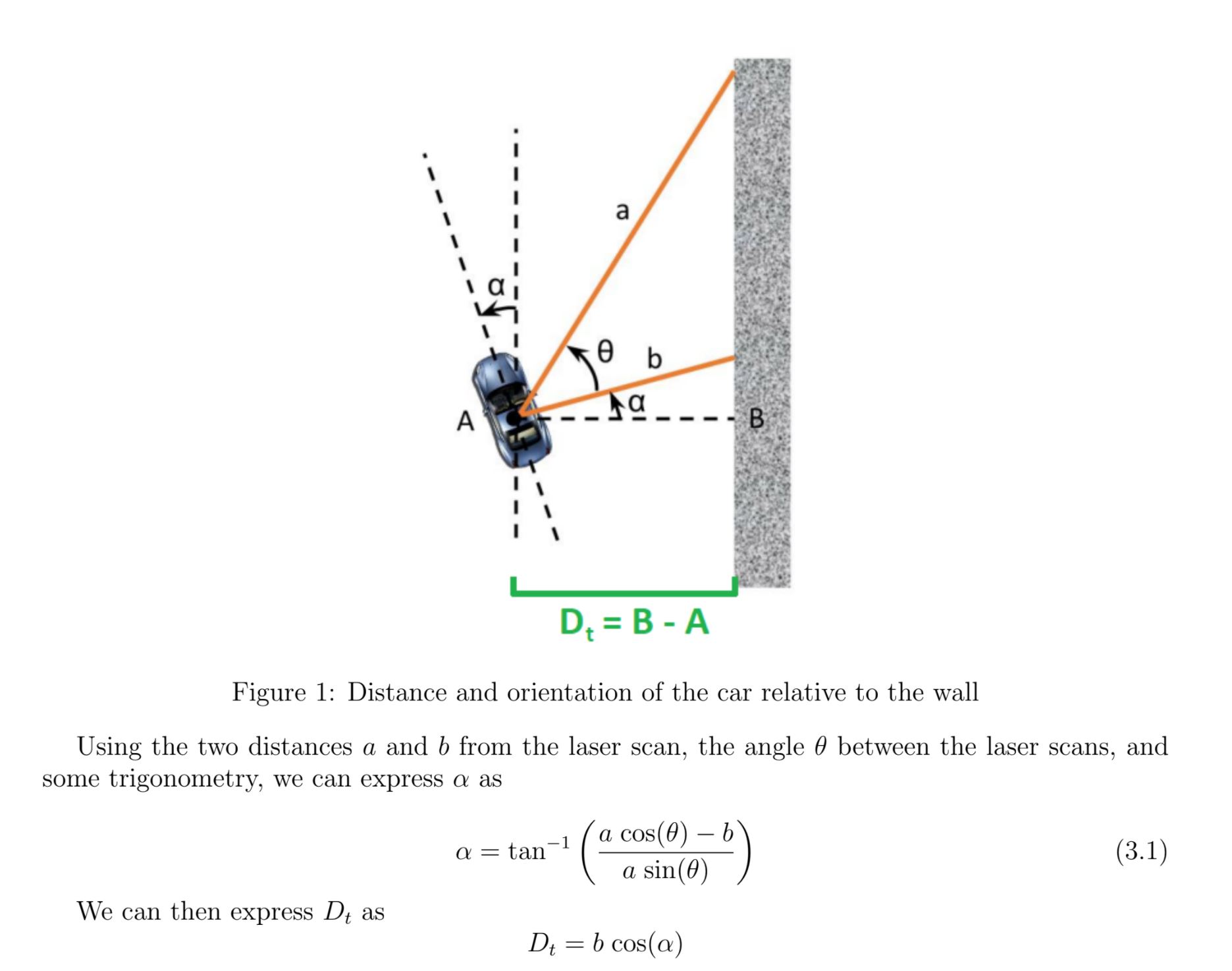 Calculation of vehicle's distance to the wall
I then applied PID control to its steering wheels to maintain the desired distance.

where the error term e(t) is the difference between the desired wall distance and the actual wall distance calculated previously. I also introduced a “distance delay” in order to account for time delay between perception and control. More technical details can be found in the below prompt document:
However, given the nature of a single PID controller, I have to tune the parameter precisely so that the car can complete a loop. If the parameters are not well tuned, it is very likely that the controller would fail in some edge cases. See the failed case here:
In fact, even if the parameters have been well tuned, this simple controller could still fail in some extreme cases. Therefore, I am going to explore more sophisticated Planning and Control methods in the future labs.
My source codes for this lab can be found on github through this link.
Reference
The lecture video can be found below:
F1Tenth Autonomous Racing Cars - Lab 2 (Automatic Emergency Braking)
During the Spring 2021 semester, I joined the F1Tenth team at Penn to conduct an interest project on multi-vehicle coordination. To get prepared for the project, I self-learned and completed Lab 1, 2, 3, 4, and 6 of the “F1Tenth” course.
Overview
This post contains my results for Lab 2, where an automatic emergency brake is implemented for the race car so that it will be stopped before crashing into anything. See the video below for a demonstration of the automatic emergency brake:
Demonstration
Procedure
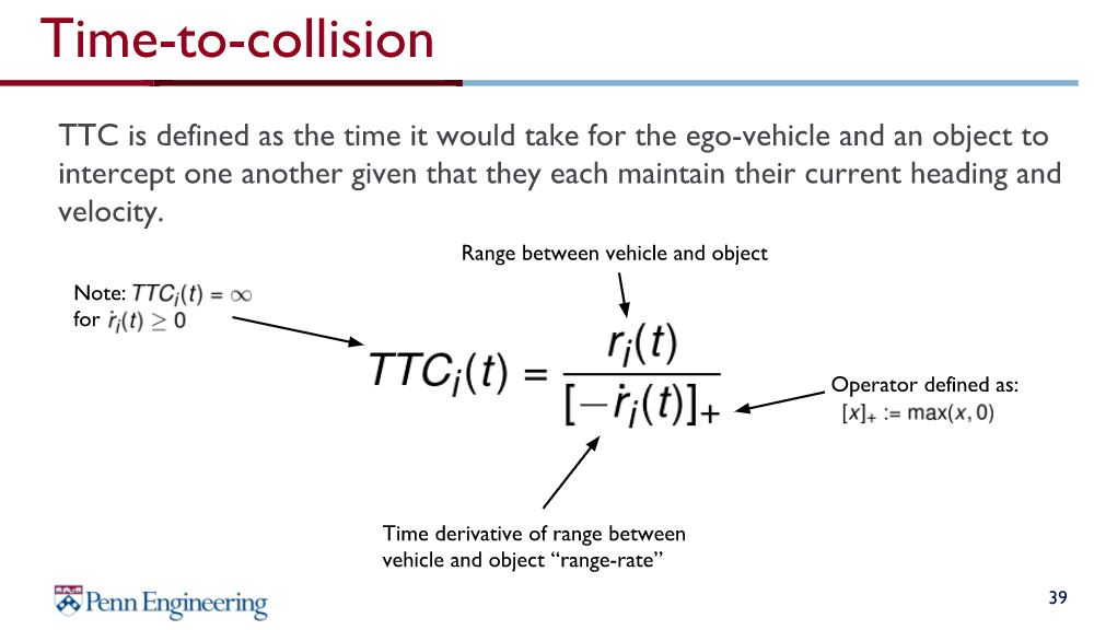
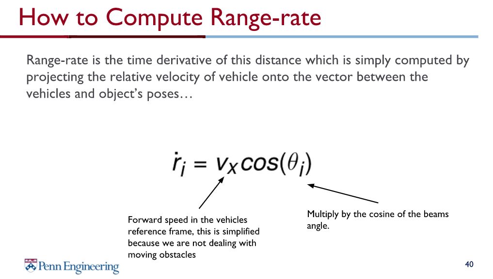
I predicted the vehicle’s time to collision (TTC) in all directions with its current motion (from its odometry information) and its distance to obstacles (from the 2d-lidar scan information). The automatic emergency brake will stop the vehicle if the minimum TTC is below a certain threshold. The slides below shows the equation for calculating TTC:
More technical details can be found in the below prompt document:
My source codes for this lab can be found on github through this link.
Reference
The lecture video can be found below:
F1Tenth Autonomous Racing Cars - Lab 1 (Introduction to ROS)
During the Spring 2021 semester, I joined the F1Tenth team at Penn to conduct an interest project on multi-vehicle coordination. To get prepared for the project, I self-learned and completed Lab 1, 2, 3, 4, and 6 of the “F1Tenth” course. This post contains my results for Lab 1, where the general concepts of ROS are discussed and explored.
The prompt document for this lab can be found below:
Here are my answers to the questions:
My source codes for this lab can be found on github through this link.
Island Beach State Park, New Jersey, USA, 2021 Winter Break Trip
During the winter break between Dec. 2020 and Jan. 2021, I went on a short day trip to New Jersey to see the Atlantic. Despite the cold weather, the Island Beach State Park has fascinating scenaries and is definitely a suitable place to visit while maintaining social distancing.
Lane Detection for Autonomous Driving
This is the open-ended final project I conducted for the course CIS 581 “Computer Vision & Computational Photography” at the University of Pennsylvania. My collaborators on this project are Han Shao, and Ying Yang.
For the general information and demonstration of results for this project, please see the following video:
More technical information is introduced in this report:
I am currently working on integrating this work to realize autonomous driving in CARLA, while designing and implementing a planner and controller to complete the loop.
Philadelphia, Pennsylvania, USA
I live in Philadelphia for my Master’s degree in Robotics at the University of Pennsylvania. In spite of the global pandemic of COVID 19, I still got a few chances to wander around the city of Philadelphia and take photos to record my moment here.
Creating Digital Twin Models for Tobacco Drying Processes
This is the capstone design project I conducted for the course VE 450 at Shanghai Jiao Tong University. My collaborators on this project are Shiyu Liu, Mengtian Guo, Tianchun Huang, and Jingyu Su.
Goal
The goal of project “Creating Digital Twin Models for Tobacco Drying Processes” is to develop multiple models for the tobacco drying process that could be combined and cross-validated with each other. When travelling through the rotary dryer, the tobacco leaves are heated by air flow through the cylinder and by conduction of heat from the dryer walls. There are a couple of controllable variables in this process: the air moisture content, the air temperature and speed insidethe cylinder, the rotation speed of the dryer, and the temperature on the cylinder walls. Furthermore, the mass of tobacco leaves inside the dryer, the initial moisture content and temperature propagated from the previous manufacturing process, are also influential to the resulting tobacco moisture content. Referring to the prior works and approaches for modeling industrial drying process, we extend our study with three methods, first principle modeling, data driven modeling, and finite element analysis. Our main objective is to exploit the correlation between the output moisture content in tobacco leaves and the factors involved in the manufacturing process through the above modeling approaches. These models need to provide good fit to the data collected from the real manufacturing environment, and they should be cross-validated with each other. An accurate and robust digital twin makes it more efficient to try out possible improvements on the system of interest, and make performance evaluations within shorter time span and lower cost.
An obstacle we have to tackle with is that, to the best of our knowledge, a tobacco drying process model with sound theoretical base has not yet been published in literature or applied under an industrial setup. We therefore have limited access to the existing methods presented on this topic, nevertheless, this is where our novelty lies in. Over the years, the tobacco drying process relies on manual control. Although PID controllers are widely applied to adjust variables such as vapor pressure, and temperature on the dryer walls, they are proved to be less efficient than trial and error in terms of top level implementations that accommodates the entire drying process. The reason primarily stands out is the time delay of the dryer system, which makes it impossible for conventional PID controllers to get real time response as feedback. During recent years, machine learning has been extensively applied to numerous tasks and achieved significant performance gains. We have noticed several works that employs ANN or deep neural based approaches to optimize the operational flow in drying process. In this project, we would like to exploit the modeling task from this direction. Finite element analysis (FEA) is frequently adopted in modeling works, which provides reliable results and pleasuring visualization without the need to address the dynamics from the aspect of mathematical/physical principles. So far, there hasn’t been a tobacco drying related work using FEA for modeling. We think this is an interesting field to explore, and the modeling results from FEA can provide valuable sources for cross-validation.
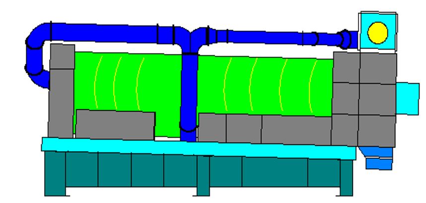 Schematic of the roller of the tobacco drying system.
Requirements & Engineering Specifications
Relevant information was collected from various sources including literature review, benchmarking products and interviews with stakeholders, Dr. Siqi Zhu from Hangzhou AIMS, Inc. Key challenges of this project lie in the demand of high accuracy of the models.
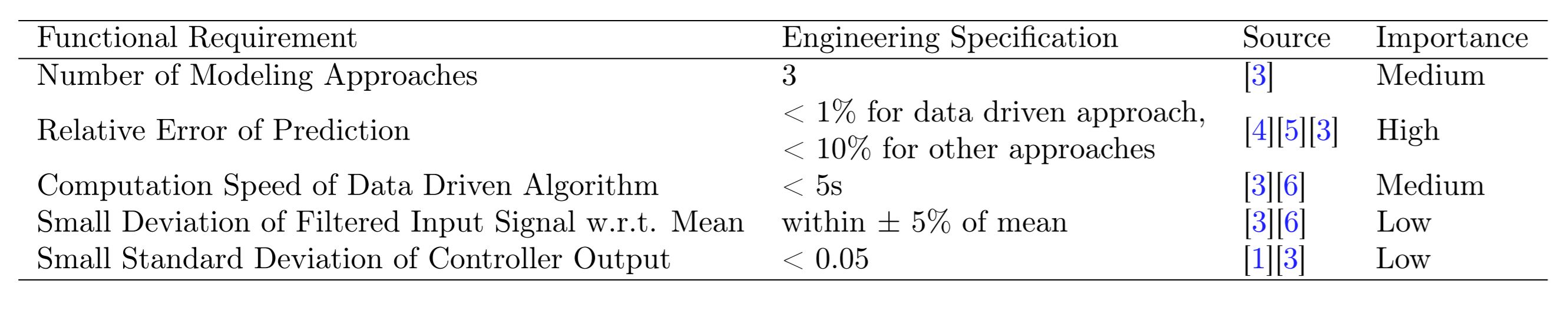 The requirements and their corresponding importance as well as engineering specification associated with the digital twin models.
Concept Generation
Figure 3. shows our concept map for this project. Our concept generation process is driven by the customer requirements, referring to how can we solve the problem and meet all the requirements.
There are mainly three parts in the concept map. The blue part specifies the concepts related to methods. The core idea of our method is to build a function that predicts the output tobacco moisture content based on system parameters. We came up with sub-concepts, first principle, data driven, and finite element analysis, indicating major directions we may try to build the target function. We then refer to literature in those directions and generate more detailed concepts such as LSTM for data driven.
Another critical part in our concept map is applicability in industry, which is colored in green. Since this project is highly related to industrial products, we introduces the concept of applicability, which further means fast response of the model and an option task to design a controller that will relate the model with actual production. One major concern of applicability is reliability. Three concepts including stability, noise rejection, and cross referencing related to reliability are then generated.
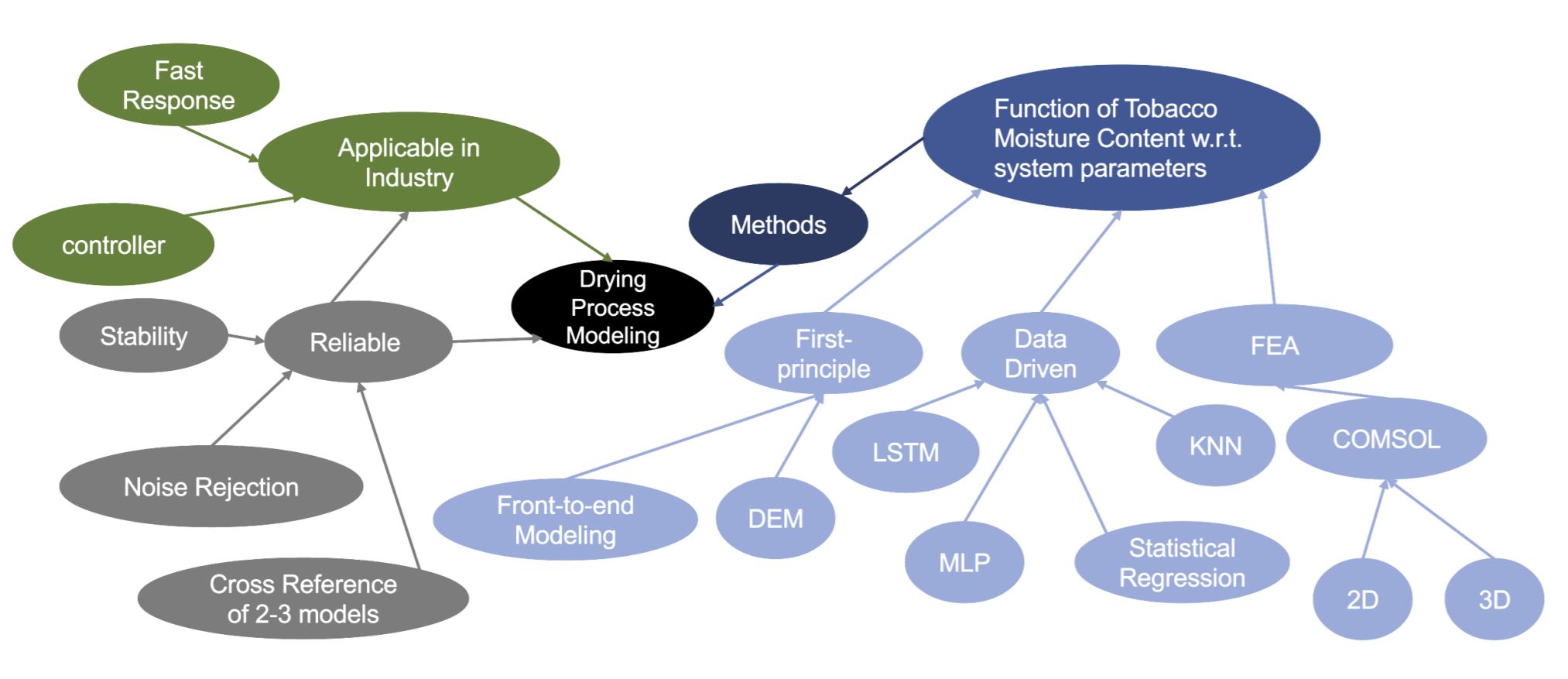 Concept map of the digital twin model. Different influential aspects are distinguished with colors, and the methods leads to three directions of concepts.
Final Design
Our final design includes three parts:
First Principle Based Method
We employ discretization in first principle modeling, which splits the whole rotary dryer into N control volumes. The output of one control volume becomes the input of the next and we assume that there are no changes on drying conditions and characteristics of gas and particles in each discretized unit. To describe the drying process happens in the ith unit, we take heat and mass transfer into consideration and derive four major equations. Those four equations connect the (i + 1)th control volume with the ith one, and we solve for quantities such as temperature and moisture in the (i + 1)th control volume based on the system of equations.
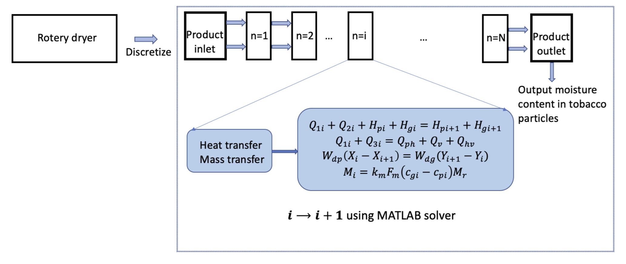 Concept diagram for first principle based method.
Finite Element Analysis Method
Due to the limitation imposed by the Finite Element Analysis method and the problem setup, we could not simulate the real situation where thousands of tobacco leaves moves inside a cylindrical roller. Therefore, we made a major simplification to the simulation: we fix the tobacco leaves in the cylindrical roller, that is, we keep the tobacco leaves stationary and pass hot air through the roller. Although this will result in deviations from the real scenario where the tobacco leaf travels through the roller, experiencing different evaporation rates at different time stamps, the simplified case should still be able to give us a reasonable understanding of the drying process and predict the general trend. We set a target tobacco leaf to be of our main interest and we place it in the middle of the roller to obtain the most averaged result. Two strips of tobacco leaves are placed at each side of the target tobacco leaf to simulate the influence of surrounding leaves to it. Since tobacco leaves are continuously supplied during operation and they occupy almost the whole length of the roller, the two strips of tobacco leaves span across almost the entire roller. Considering that the gaps between the target tobacco leaf and the tobacco leaf strips are small, the effect of them could be neglected. After verification with simulations, we simplify the model to the one shown below with a single long tobacco leaf strip. In this case, the target result becomes the moisture content at the center location of the tobacco leaf strip.
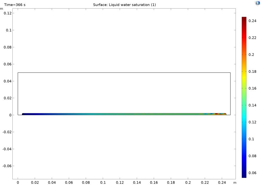 COMSOL model and simulation results for the Finite Element Analysis method.
Another major simplification is the size of the roller: it is brought down to 0.25m in length and 0.05m in diameter for the 2D model instead of the true size which is 10m in length and 3m in diameter. This is due to the limited computing power we have. Since we keep the target tobacco leaf true to size, the roller would be thousands of times larger than the tobacco leaves in size, this will require incredible long time to run the simulation. Therefore, we change the roller to a smaller size. We note that this change in size will also create deviations from the actual scenario, but the simplification is necessary for the completion of the Finite Element Analysis simulation.
With an understanding of the system physics, we propose 4 Physics modules to simulate the dynamics inside the drying process: Laminar Flow, Heat Transfer in Fluids, Transport of Diluted Species: Liquid Water, and Transport of Diluted Species: Water Vapor.
Laminar Flow module simulates the flow of the hot air over the roller’s wall as well as the tobacco leaves. Laminar flow instead of turbulent flow is selected here because the Reynolds number Re = 203397 < 500000. Since the pressure has great impact on the rate of evaporation for water vapor, the simulation of air flow is important.
Heat Transfer module simulates the heat transfer between the hot air, the tobacco leaves, and the roller wall. It also simulates the heat transfer inside the materials themselves. Since the temperature has great impact on the rate of evaporation for water vapor, the evaluation of the heat transfer is essential.
Transport of Diluted Species: Liquid Water simulates the movement of liquid water inside the tobacco leaves. The concentration of liquid water is also influential on the rate of evaporation for water vapor, so this module is nonnegligible.
Transport of Diluted Species: Water Vapor is the essential module in this model because the drying of the tobacco leaves is achieved through the evaporation of water vapor.
These four Physics modules are coupled in COMSOL Multiphysics to perform simulations. The laminar flow is first simulated using stationary solver to achieve the equilibrium state, the other three modules are then solved by time dependent solver. The simulation time is set to be the estimated travel time of a tobacco leaf inside the roller, which is 366 s. The resulting water saturation, or moisture content of the target tobacco leaf is then the desired result of the simulation.
Data-driven Methods
Here we implemented a model based on Long Short Term Memory (LSTM) neural network that can predict the output moisture content at the next timestamp given any timestamp with its previous outputs and parameters. The metric we used to evaluate the model is the average relative error between the predicted outputs and actual outputs from test data sets. An overview of the final design is shown in the flow chart below. The procedure includes preprocessing the data, training the model, and validating the result.
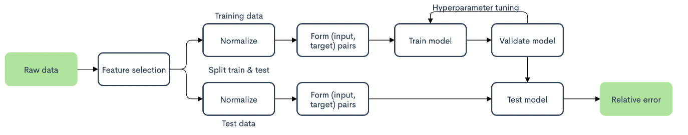 An overview flow chart of data-driven methods.
General Validation Process
Each model is validated by inputting the parameters in the provided data set and comparing the resulting output value with the ground truth data. The resulting computed accuracy of the models should stay within the engineering specifications defined above. Other engineering specifications are also validated to be satisfied where appropriate.
Performance (by simulation)
The models were generally able to meet the specifications as shown below.
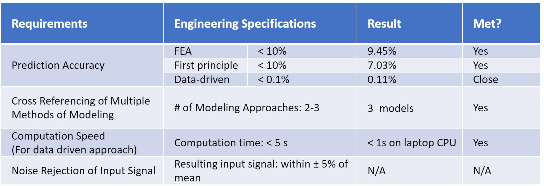 Performance of the models.
Future Improvements
First Principle Based Method
The design based on physical dynamics of the drying process requires the knowledge of the tobacco physical properties, heat and mass transfer characteristics, and the motion dynamics caused by the rotation of the drum. Since this project is at its initial phase, we are not provided with data that can only be acquired through experiments in lab. Thereby, our model heavily relies on parameters and empirical equations stated in literature we referred to. We also make assumptions on dimensions and other physical properties of the rotary drum due to the lack of measured data. During the implementation process of our first principle based model, we find that an accurate description on the physical properties and motion dynamics is very essential to build a digital twin model close enough to the real manufacturing process. We hence recommend the project team to verify the property data with experiments in lab and measurements in factory as future efforts to further enhance the accuracy and robustness of the model.
Finite Element Analysis Method
Similar to the first principle based method, the Finite Element Analysis model heavily relies on the parameters assumed or stated in literature we referred to. The variation of these parameters can create large variations in the simulation results. Therefore, it is important and recommended to verify the property data with experiments in lab and measurements in factory to further enhance the accuracy and robustness of the model. Furthermore, due to the limited computing power, the FEA model is only implemented for the roller with reduced size. If additional computing power is available, it is recommended to run the simulation with the roller true to size, which will provide more reliable results.
Data-driven Method
Neural network is not the only method to deal with such kind of problem, traditional machine learning methods including K-Nearest Neighbours (KNN) and Random Forest or traditional statistical methods such as Autoregressive Integrated Moving Average (ARIMA) model can also be used to solve the regression problem. In our experiments, KNN leads to comparable result to LSTM model, while the model is still not fine tuned. Therefore, after tuning these models, better results could appear. Furthermore, since these models are theoretically different, they may not result in the same kind of bias as the LSTM model. A better method in the end would be an ensemble model which consists of several model like the Random Forest Regression, which gives a promising result without much fine-tuning as follows:
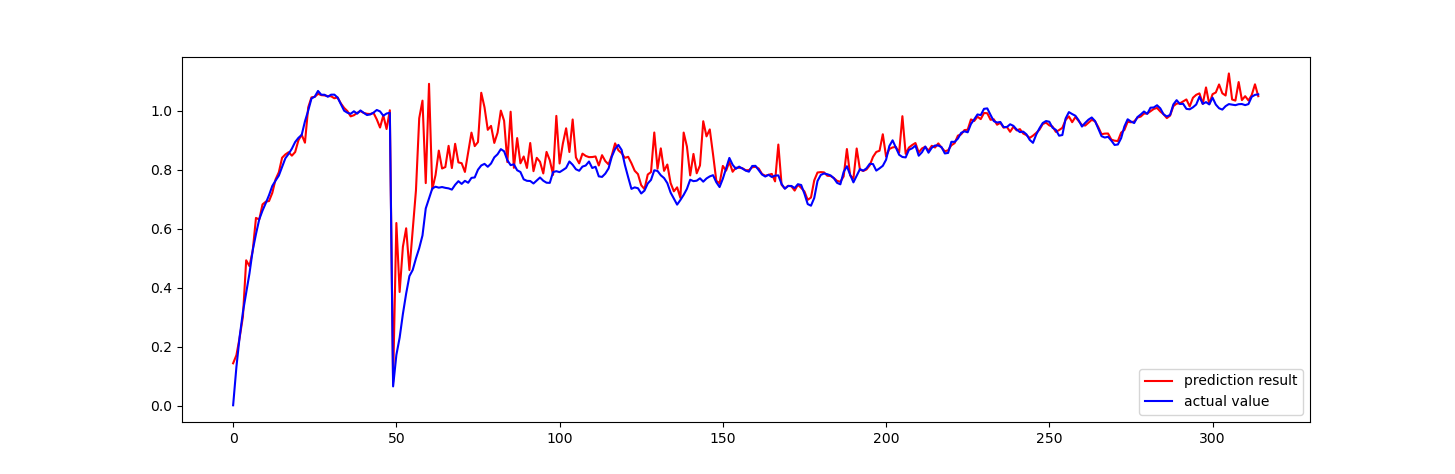 Moisture prediction result of Random Forest Regressor.
Another model that can be explored is the ExtraTrees Regressor, which is an enhanced version of Random Forest algorithm that introduces randomness into feature splitting. However in our practice, this model shows a strong sign of overfitting, so its feasibility will need further examination.
Model Integration and Future Efforts
In this project, we propose to solve the modeling task in a multi-directional manner, with each method having its own features and limitations. First principle based modeling has a robust nature since the heat and mass transfer properties are studied in the dynamic system involving gas-particle flow, whereas it cannot predict the output moisture content in tobacco leaves with high precision. Finite element analysis provides appealing and straightforward visualization that monitors the real-time status of the tobacco particles inside the drum, while this method suffers from expensive computations, and it does not take the complex particle motions into consideration. Data-driven method learns to predict the outlet tobacco moisture by investigating the correlations among measurements in the industrial environment, and gives the most accurate and precise results we have so far. However, the model is likely to fail once the manufacturing conditions are changed.
Model integration is a possible next-step for this project, where a strategy to post-process the results given by our models is studied. It can be as simple as finding the mean of these values; or as complicated as training neural networks that predicts on the weights to be assigned to each model and eventually calculate the weighted average as the final result. Moreover, the cross-validation between the established models can provide more comprehensive examinations on the capability of the models developed from each direction. The existing data we have only varies within a small margin, while cross-validation extrapolates the manufacturing conditions to a broader range. Though we are not able to finish this part within the time span of the project, it is genuinely an interesting field to exploit as future work.
The figure below demonstrates our rough idea on how our modeling work could contribute to product quality improvements by optimizing the manufacturing process. The digital twin models can provide a platform for the vast searching and trials among the rational range of inputs and controllable variables. Each of these models will be assigned to a weight as described above, thus the outlet tobacco moisture content can be calculated under every given condition. The data recording the conditions and corresponding results will form a dictionary, which can be referred to when the input variables and target output moisture content are known. In this way, the optimal values of the controllable variables can be found, and eventually deployed to lower-level controllers to confine the outlet tobacco moisture content within a small error margin.
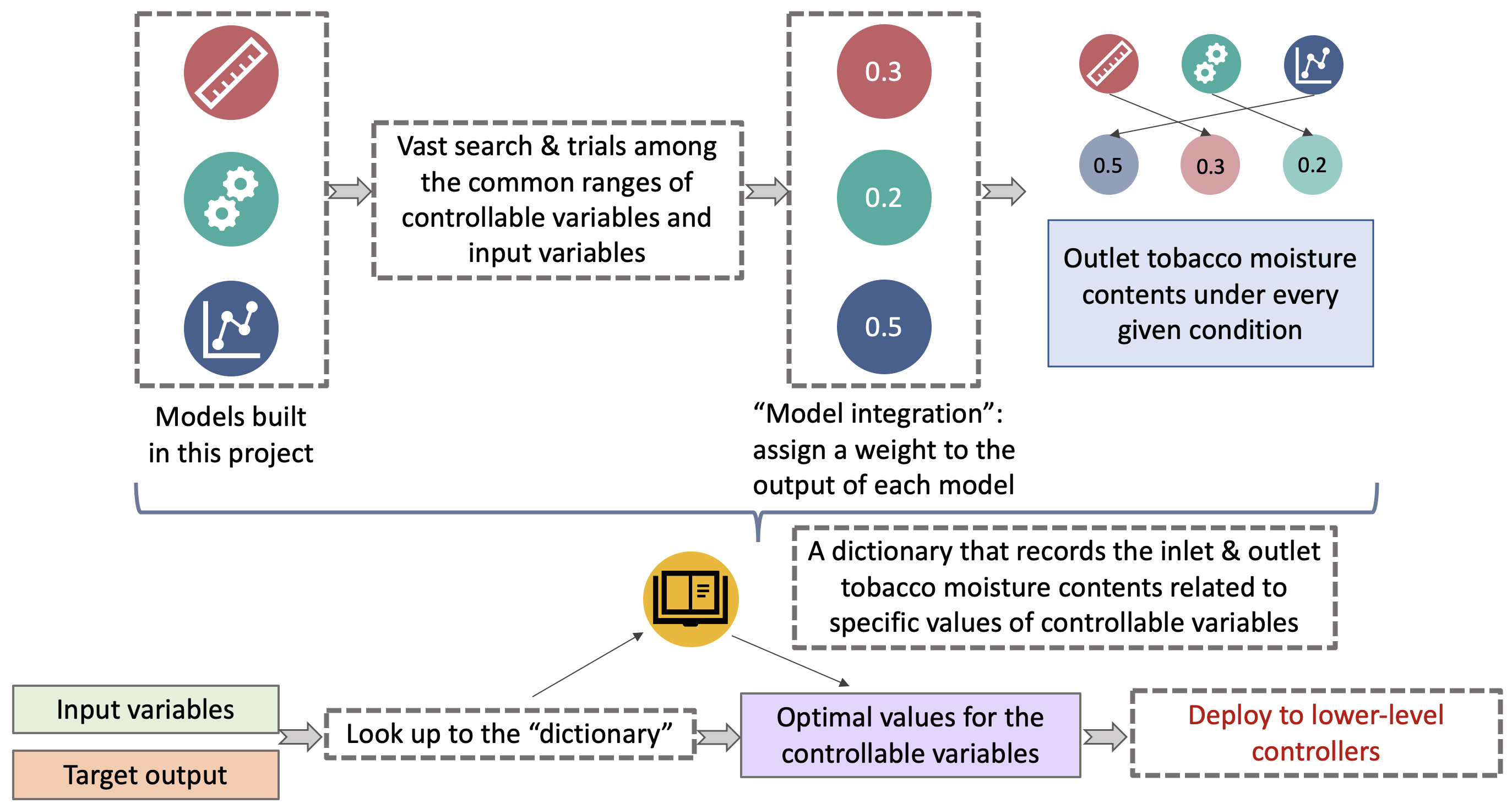 Model integration and future efforts.
Conclusions
Our project aims to create digital twin models for the tobacco drying process, a task rarely explored by either the industry or the academia. Referring to the existing methods that have been adopted in related industries, we propose three approaches: first-principle modeling, data-driven modeling, and finite element analysis. From the perspectives of first principle based modeling, FEA, and data-driven modeling, discrete element method, 2-D FEA, and LSTM network demonstrate the best compatibility to the design requirements respectively. We therefore adopt the selected approaches to develop our final design. All of the three models reach satisfying relative errors (7.03% for first-principle, 9.45% for FEA, and 0.11% for data-driven) that is lower than the engineering specifications. However, each of the three models also has its own limitations, e.g. the FEA simulation makes significant simplifications and there is unsolved problem related to heat transfer in first-principle based modeling. Further improvements are needed and assembling the three models to reach a more reliable model will be an interesting future work. In summary, our project meets the main requirements of developing accurate models for tobacco drying process using three distinct methods.
Our major contribution in this project is to build up a framework for drying process modeling in tobacco industry. To the best of our knowledge, there is no existing work that provide a systematic view of the drying modeling using the three proposed methods. Our work can therefore provide reference for future drying process modeling. The methods we used can be extended to other drying process such as the modeling of the moisture change of tobacco bulk.
Acknowledgements
We would like to acknowledge our sponsor Zhiqi Zhu from AIMS, and instructors Shouhang Bo, Mian Li, Chong Han, and Jigang Wu from SJTU-JI for their kind help along the way. They have faced with more obstacles than us during this semester while still provided our team with timely suggestions during lectures and meetings. Even though the modeling project requires a large amount of knowledge basis on fluid dynamics and thermodynamics, which most of us are not familiar with, we learnt a lot from this project and on how to overcome challenges. We would like to extend our gratitude to every team member’s contribution and to sponsor’s and instructors’ support.
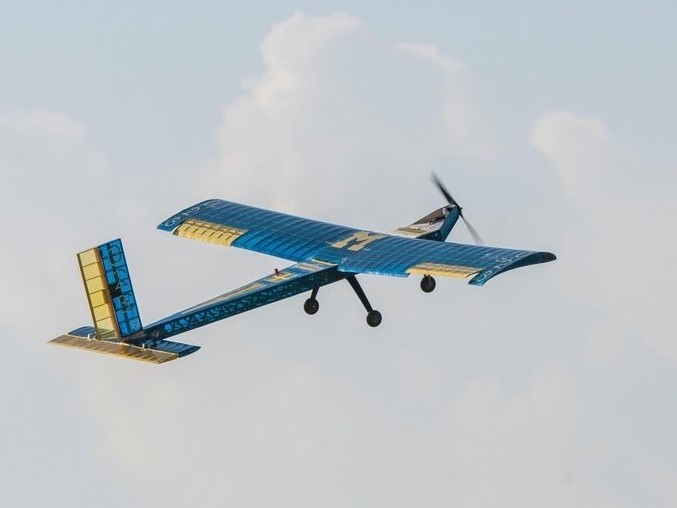
SAE Aero Design East (M-Fly Aerodynamics Sub-team)
This is a student team project I joined for two years when I was at the University of Michigan. The student project team was called the M-Fly Student Aero Design Team. It was a fun, strong and passionate team where we collaborated well in an organized manner.
The following are the two aircrafts that I was mainly involved in designing during my two years on the team.
I worked on the M-11 as a member of the aerodynamics team of the aircraft, where I mostly learned and worked with Forster Guo, the aerodynamics lead at that time.
 M-11
M-11
 M-11
M-11
During my second year on the team, I was elected as the aerodynamics lead for the M-12. Therefore, I taught and led a sub-team to design the aerodynamics aspects of this new plane throughout the year.
 M-12
M-12
 M-12
M-12
 M-12
M-12
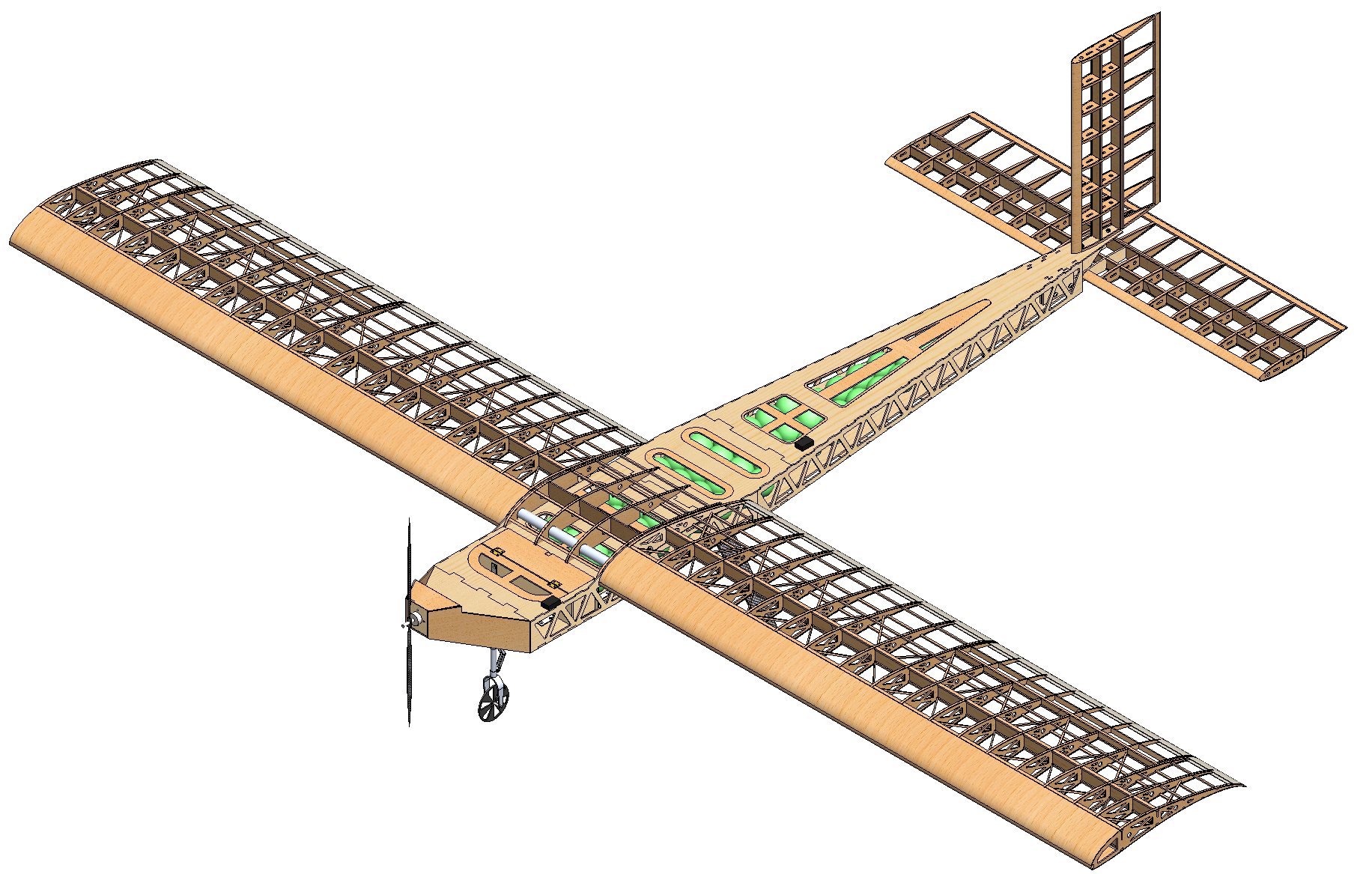
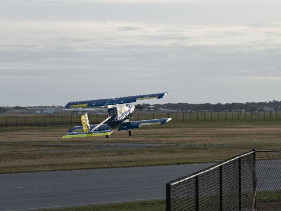
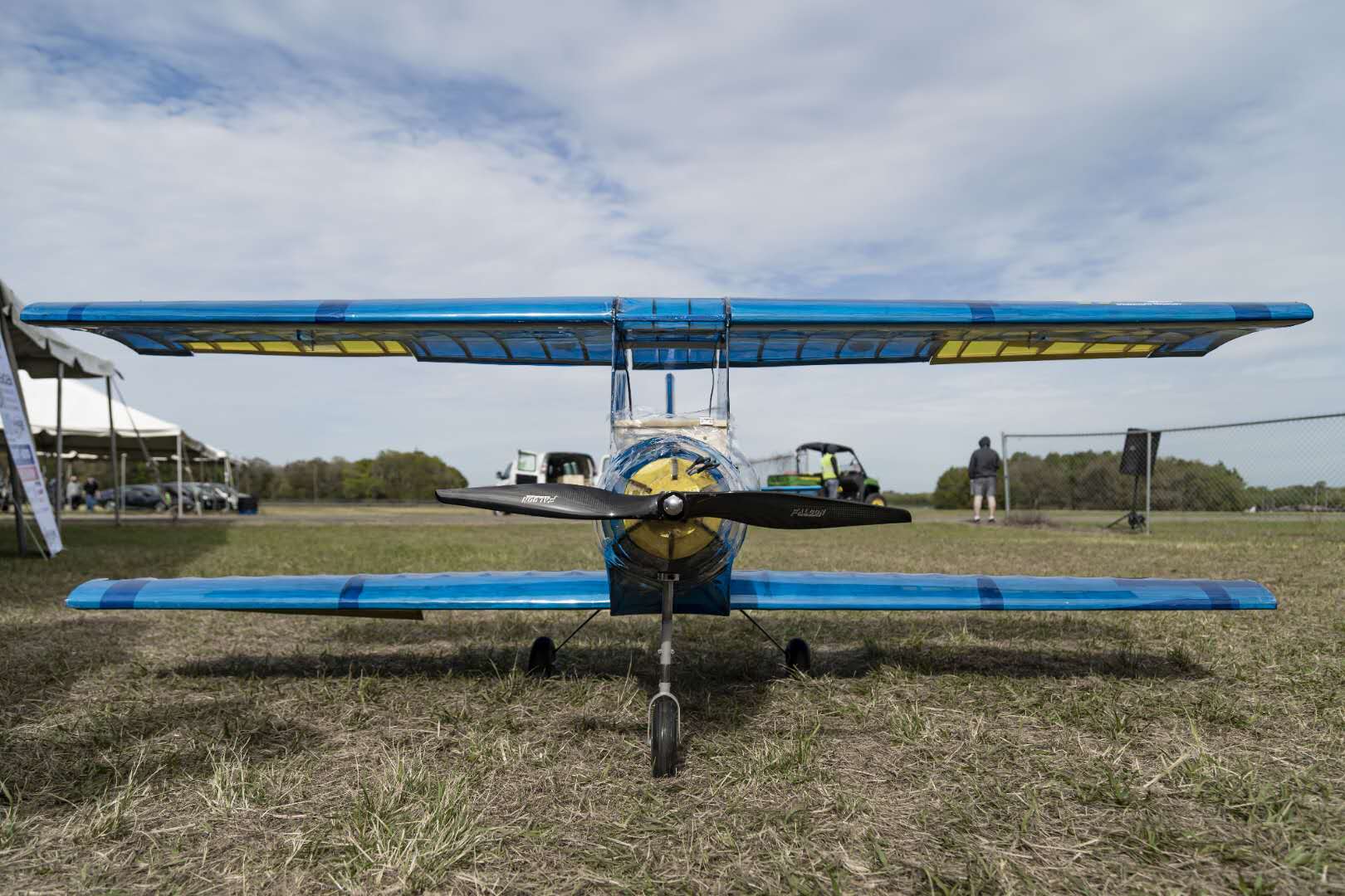
I am going to introduce the aerodynamics design of the M-12 below since this is the aircraft that I am mostly responsible for and spent the most time on as well. This is also the first biplane at this size on the team’s history as well! We were all excited that it successfully flew a few rounds during the 2020 SAE Aero Design East competition in Lakeland, FL.
Goal
Critical to M-Fly’s performance at SAE Aero Design East 2020 is the ability of the M-12 to record three flight rounds carrying 22 lbs of boxed payload and one spherical payload. Additionally critical to the team’s success is its ability to score within the top five teams in the design report and presentation respectively to maintain competitiveness with the other teams.
Overall Design Layout & Size
The M-12 is a bi-wing aircraft with its bottom wing positioned low, and its upper wing placed high above the fuselage and staggered forward of the bottom wing. Both wings utilize the Selig S1223 airfoil, and its planform and taper were designed to maximize payload weight capacity and to reduce wingspan given the maximum static thrust available. The conventional empennage layout was seleced to aid in manufacturability and due to weight savings over alternatives. The vertical and horizontal portions of the tail employ the NACA 0012 symmetric airfoil. A 199 Kv electric motor that produces 15.65 lbs of static thrust with its 24 in by 16 in wooden propeller is used along with a tricycle configured landing gear system.
Optimization and Sensitivity Analysis
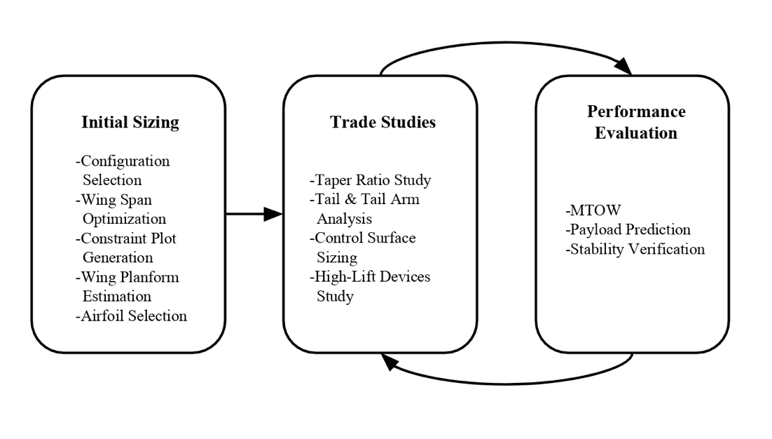
Initial sizing of the M-12 was conducted based on data from past years, initial model estimations from AVL, as well as wingspan and configuration analysis. A biplane configuration was predicted to generate a higher flight score than a monoplane configuration. Further, sensitivity of the potential flight score was analyzed against the wingspan, and reached zero when the wingspan is 8.5 ft, maximizing the M-12’s score. The M-12 was then optimized through trade studies and performance analysis on each design variation, as shown below.
 Optimization process of the M-12.
Design Features & Details
Airfoil Selection
Around 30 high-lift airfoils were selected from Airfoil Tools and considered for the M-12. Out of them, three airfoils were selected to be the final candidates for the M-12. These were compared with their Clmax, L/Dmax and stall angle as shown in Table 1. Each airfoil was put into the team’s takeoff prediction code and analyzed with the other conditions set constant. The S1223 airfoil was found to require the shortest takeoff distance and was thus picked as the airfoil for the M-12.
 Characteristics of three candidate airfoils at Reynolds number of 500000. The selected airfoil is highlighted.
Configuration & Wing Design
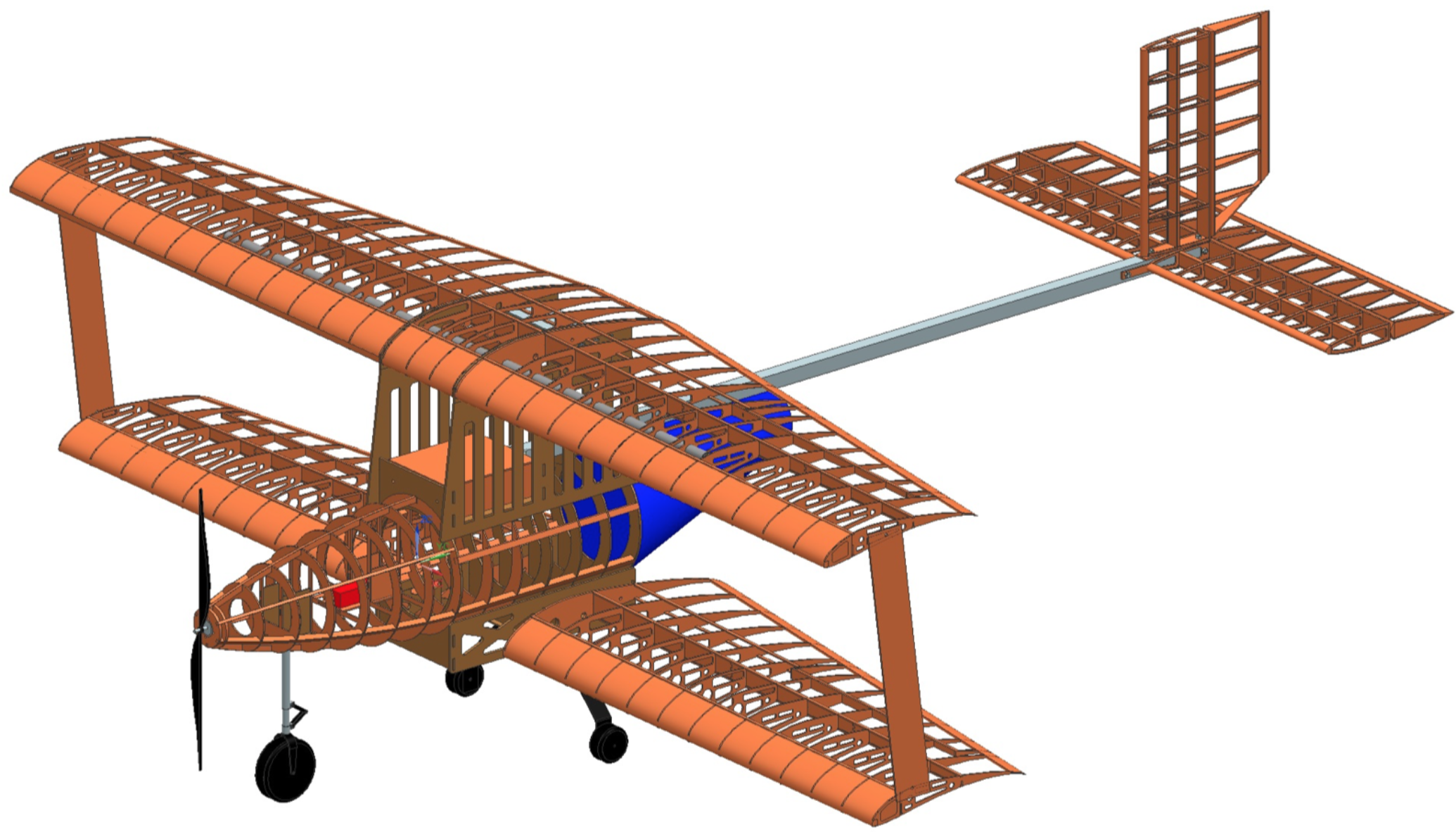
A top view of an M-12 wing is shown below, and the parameters of it are summarized in the table below.
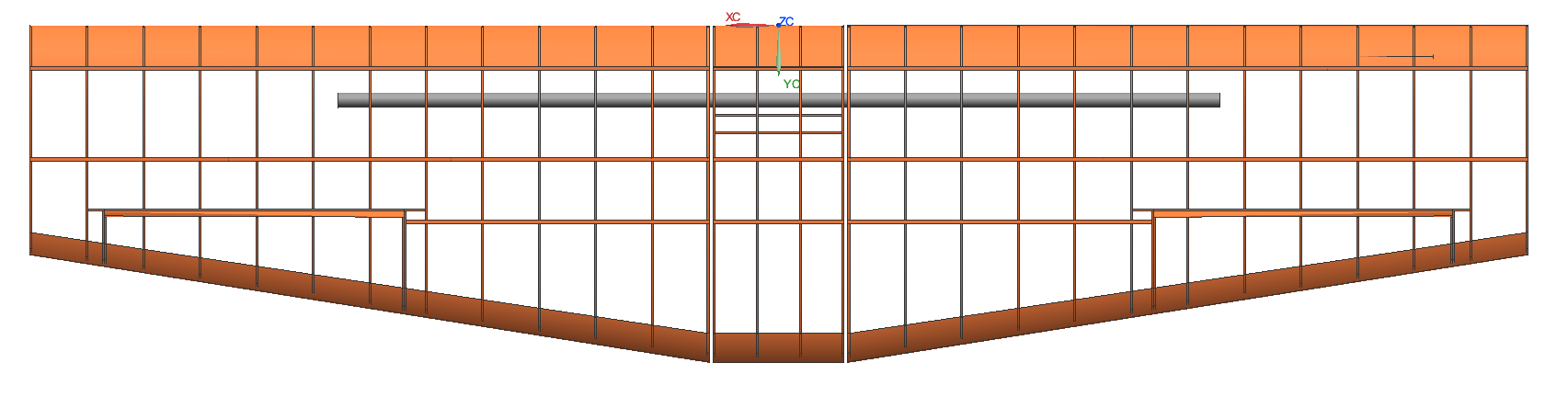 Structural layout consists of a basic rib and spar configuration.
 M-12 Wing Parameters (for a single wing).
The high-lift and short runway requirements encouraged the team to consider a biplane configuration for the M-12. Since the wingspan is also involved in the scoring equation, a scoring analysis was conducted for both the monoplane and biplane configurations at different wingspans. The analysis was based on the planform area determined from the chosen design point of the constraint plot shown later, and the results are shown below, which indicates that the M-12 will achieve the highest score at 8.5 ft wingspan with a biplane configuration.
 Scoring analysis of the M-12 for both the monoplane and biplane configurations.
The team then analyzed stagger, taper, twist and incidence angle of the wings using AVL. A stagger of 0.1 m between the top and bottom wing was found to maximize the lift coefficient through AVL analysis and was thus chosen for the M-12. Trade studies were then performed on taper ratio and taper start position. In order to maximize the lift coefficient, L/D, and efficiency while maintaining a manufacturable chord size, the taper ratio was chosen to be 0.70 and begins adjacent to the fuselage. As sweep would only be beneficial for flight at the transonic regime, it was ruled out due to the aircraft’s low expected flight Mach Number. Geometric twist was not considered for ease of manufacturability.
The control surfaces were sized using the team’s historical data and a trade study at the banked turn stage. In order to achieve small aileron deflection, the team selected ailerons located from 50% to 90% of the half span, while occupying about 30% of the chord on average. Ailerons were designed on both sets of wings and are controlled separately to allow for aileron differential that reduces yawing moments generated by the ailerons.
Empennage
The conventional tail and the T-tail configurations were considered for the M-12. The conventional tail is advantageous due to its historical credibility, ease of manufacturing, lighter structural weight and because it is less affected by wing wake, while the T-tail could reduce downwash on the horizontal stabilizer due to the biplane configuration. After comparison from simulations in AVL, the two types of tails were found to provide similar performances on efficiency, L/D, and control surface deflection. In order to achieve better manufacturability and weight savings, the conventional tail was chosen for the M-12 over the T-tail.
Trade studies were then performed on the empennage sizing in order to obtain the most efficient configuration. The tail boom length was chosen to be 4.65 ft to provide a large enough rotation angle of 17.5 degrees. Based on historical tail volume coefficients on the team, the horizontal and vertical stabilizers were sized using the tail coefficient method. Both stabilizers are untapered and unswept for ease of manufacturing.
The elevator and rudder are both 50% of the chord and span the length of their respective stabilizer. The tail has an incidence angle of 2 degrees to reduce the required control surface deflection for maneuvers.
Loads & Environments, Assumptions
Design Load Derivations
The maximum expected lift forces on the fuselage, wing, and empennage during flight and the maximum forces on the tail boom were analyzed using AVL. The load factor of the M-12 is plotted against its speed below.
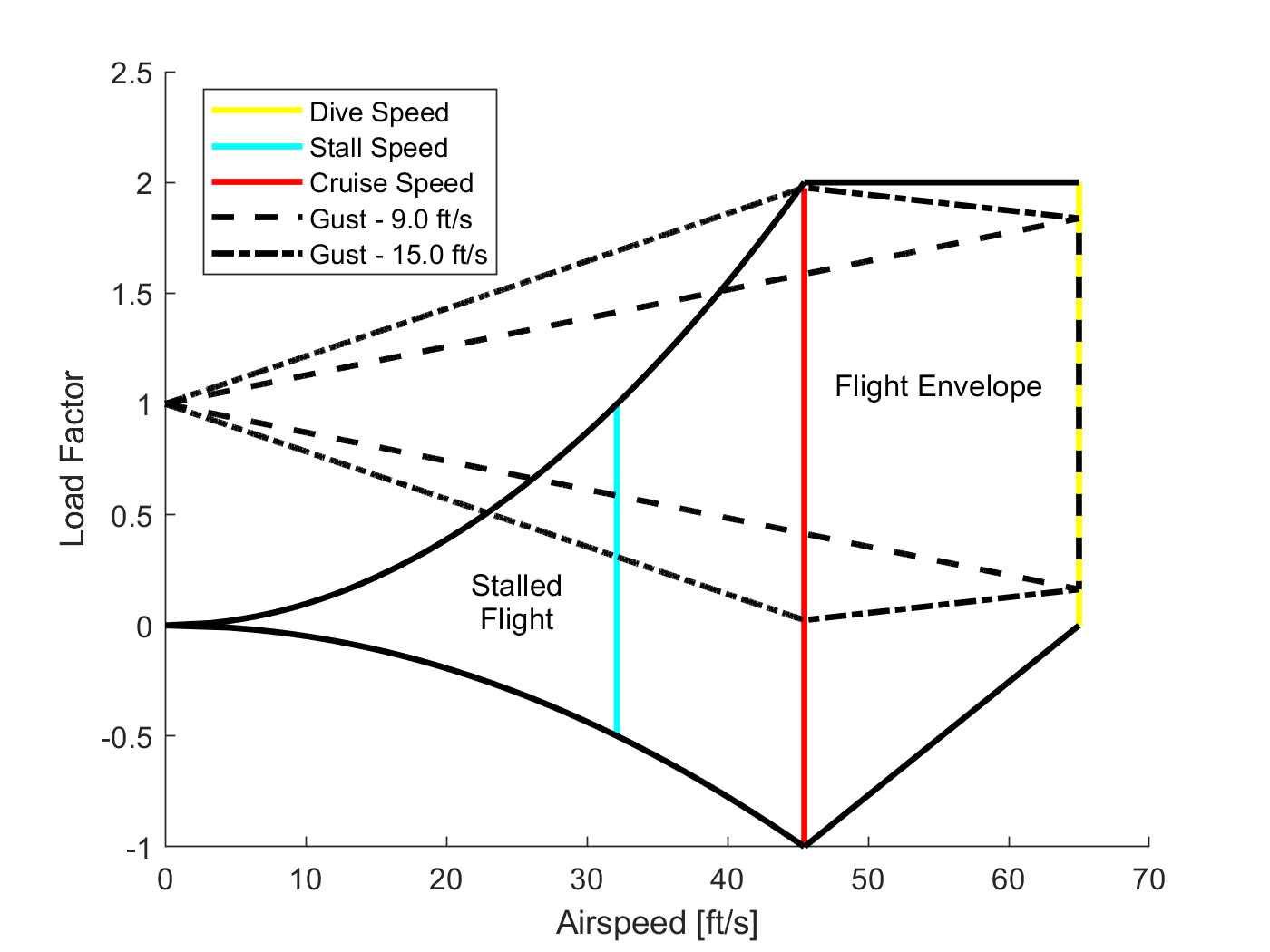 V-n Diagram of the M-12.
Environmental Considerations
The aircraft has a limited operational temperature based on the ratings of the ESC and Li-Po battery as well as air density, which is temperature-dependent and impacts maximum payload capacity. The M-12’s electronics are rated for 0°F to 113°F, and operating outside of this range incurs a power drop of around 50%. Analysis of historical weather data in Lakeland, Florida in early March leads the team to expect a temperature range between 56°F and 82°F, which is firmly within the safe operating range for the electronics. The aircraft’s UltraCote covering will prevent structural and electronics damage in the presence of high humidity, fog, and/or light precipitation. Adhesive tape is used to seal hatches and attachment points to protect internal systems. Greater precipitation and other inclement weather may damage the electronics or compromise the structural integrity of the airframe. High winds are also a concern, and vertical gusts of up to 15 ft/s are taken into account in the flight envelope as shown in the figure above.
Performance Analysis
Flight & Maneuver Performance
The flight performance parameters of the M-12 are calculated and estimated by MATLAB and AVL, and the results are summarized in the table below.
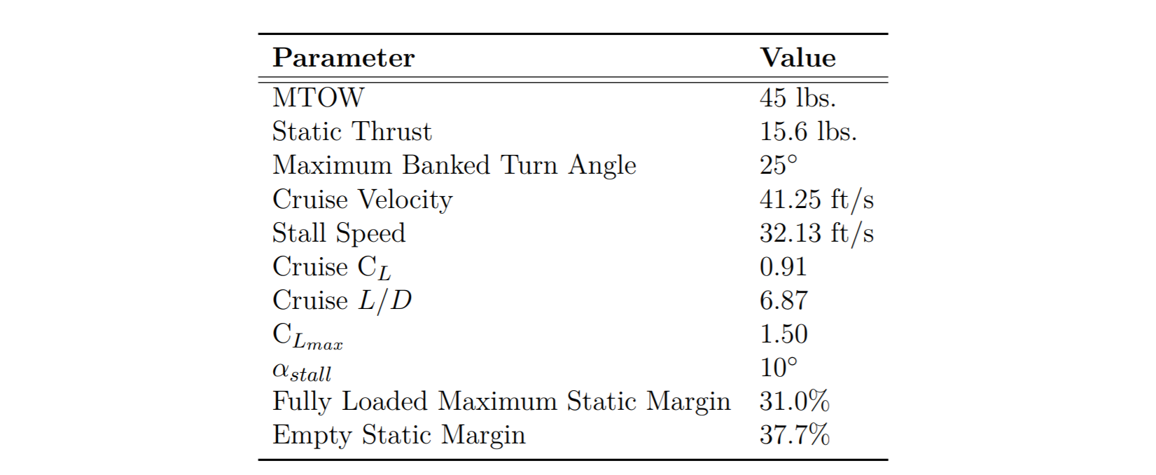 Flight performance parameters of the M-12.
The M-12 has a CLmax of 1.50, which occurs at a stall angle of 10 degrees. These values are determined by running AVL at trimmed cruise conditions and increasing the angle of attack until any section of the wing reaches a sectional lift coefficient greater than CLmax of the S1223 airfoil at the cruise Reynolds number of 500000. While the stall angle is rather low, the team is confident that the actual stall angle is higher based off historical data. Additionally, wing manufacturing can produce imperfections on the leading edge, which may trip the air flow to turbulent and in turn help delay separation and stall.
The drag polar of the M-12 was computed and constructed from AVL, as shown in the figure below. The cruise L/D was then extracted from the drag polar to be 6.87. The Oswald efficiency factor is estimated to be 0.65 at trimmed cruise condition.
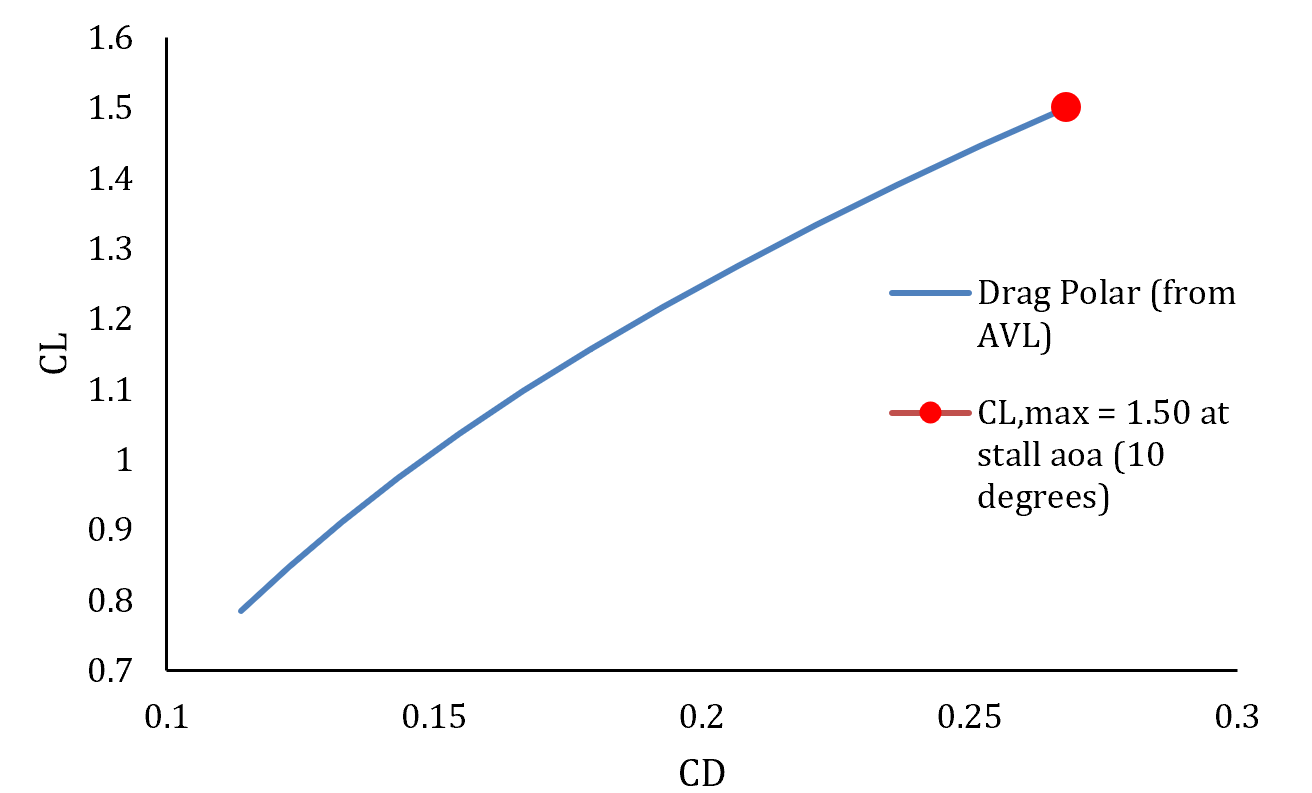 Drag polar of the M-12 constructed from AVL.
The Trefftz plot of the M-12 at trimmed cruise condition is shown in the figure below.
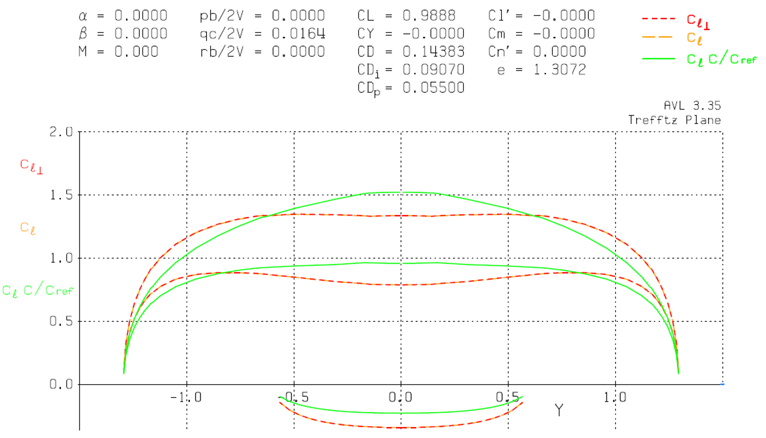 Trefftz plot of the M-12 at trimmed cruise condition.
The M-12 power requirement was calculated for various stages of flight to ensure that the aircraft is capable of completing a flight round at competition while carrying the maximum predicted payload. Weight, climb rate, air density, velocity, reference wing area, parasitic drag, induced drag factor, and bank angle in radians are taken into account to determine power requirements which were used to produce the operational flight envelope shown in the figure below. As shown in the figure, the M-12’s propulsion system provides necessary power to satisfy all major flight stages in its fully loaded configuration.
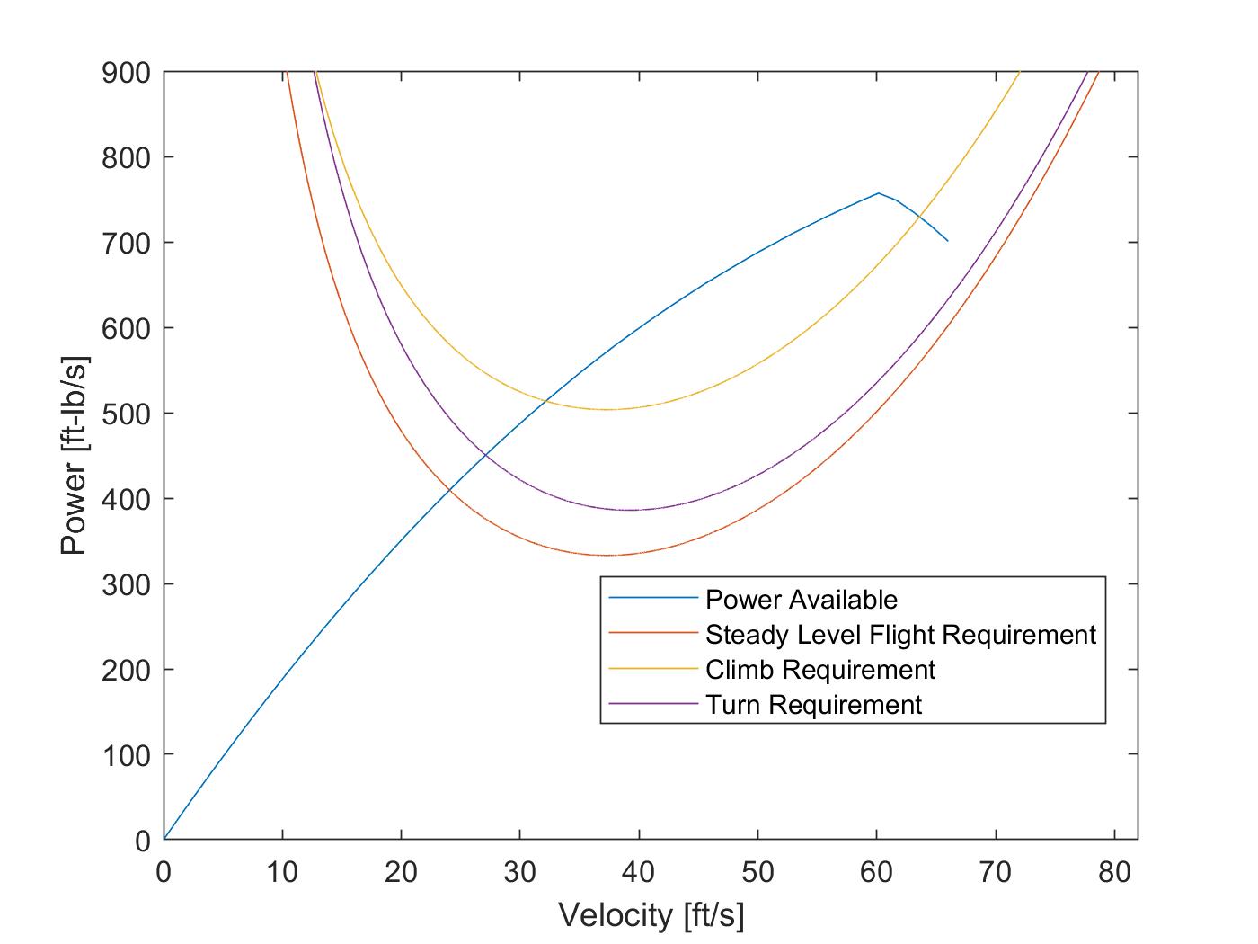 M-12 flight envelope
The thrust-to-weight ratio and wing loading constraints for stall, takeoff, climb, and cruise stages are shown in the following figure. It is indicated that the design point selected from preliminary sizing and subsequent system optimization satisfy the flight stage requirements.
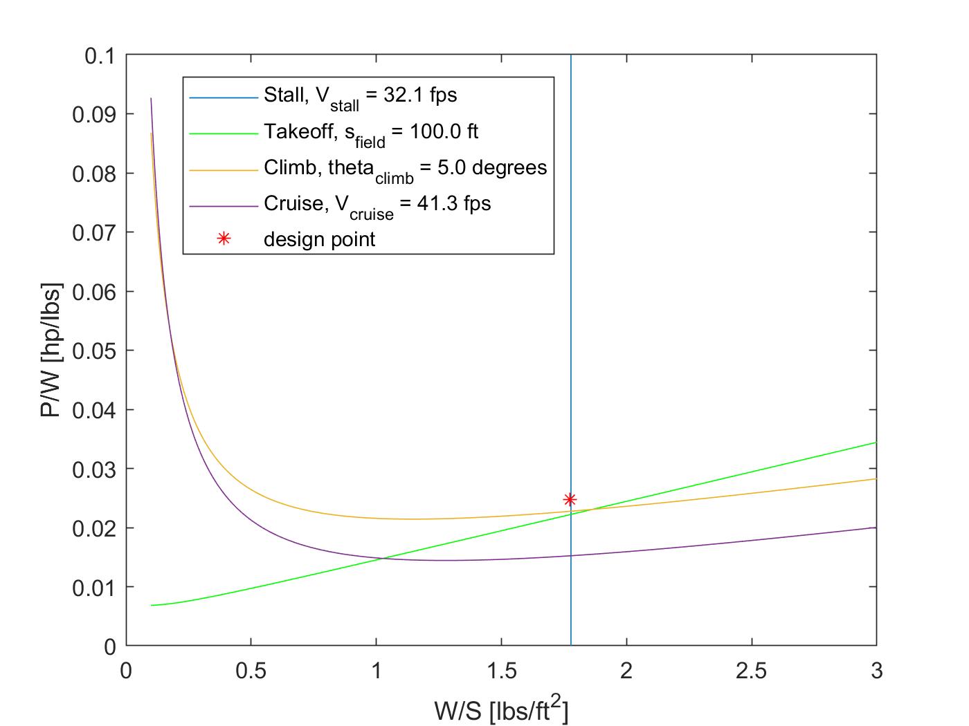 M-12 flight constraints
Dynamic & Static Stability
Stability was the priority for the M-12 design to ensure a safe flight. The empty weight static margin of the M-12 is 37.7% and the fully load static margin of it is 31%, which ensures the longitudinal stability of the plane during flights.
With the goal of achieving Level 1 dynamic stability in all modes as defined by the CooperHarper scale, the dynamic stability of the M-12 was also analyzed using AVL’s eigenmode analysis. Results are shown in the table below. M-Fly has historically found that AVL’s spiral mode is inaccurate as the team has not had trouble with spiral instability in the past, so the spiral mode was not considered here. Since the M-12 achieves Level 1 stability in all modes, pilot compensation would not be required to maintain steady level flight.
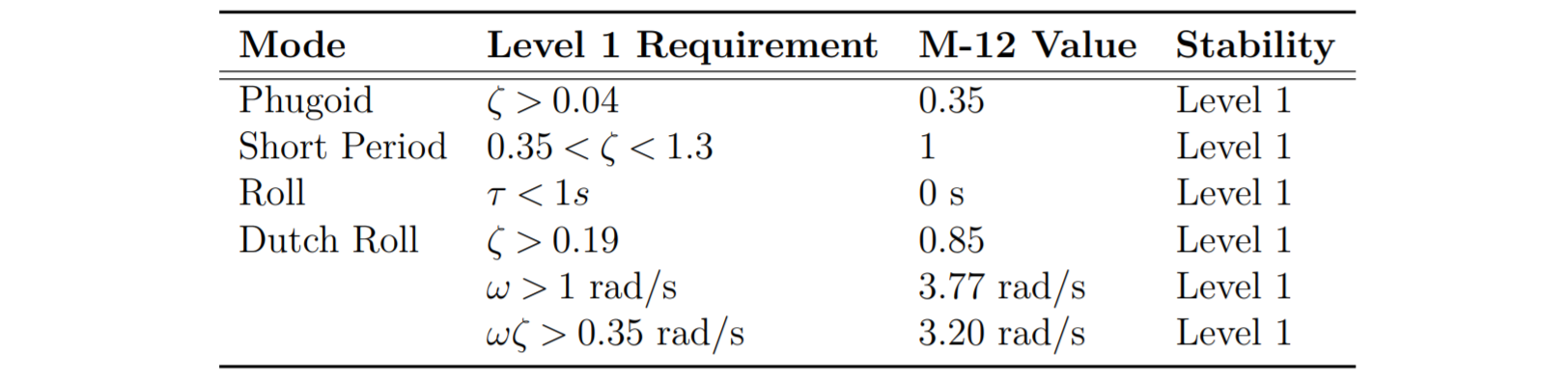 Dynamic stability of the M-12 with its fully loaded configuration.
Lifting Performance, Payload Prediction, and Margin
The lifting performance of the M-12 is presented in the payload prediction plot as shown below, taking into account density altitude, thrust, coefficient of lift and airspeed velocity. The M-12 was modeled at trimmed cruise stage at several density altitude conditions, and the lift performance was calculated by AVL. At sea level, the maximum expected payload is 22 lbs.
 Payload Prediction Graph.
Conclusion
The M-12 is a bi-wing configured aircraft using a conventional tail that has been designed to place at the top of the 2020 SAE Aero Design East competition. The aircraft has the capacity to carry one spherical payload and up to 22 lbs of boxed steel payload, leading the team to believe it will be competitive in flight rounds and in other portions of the competition.
Although the M-12 eventually did not come to the top due to power losses of the propulsion system that could not be fixed during the competition, it successfully flew a few rounds in the air and proved the feasibility of our design.
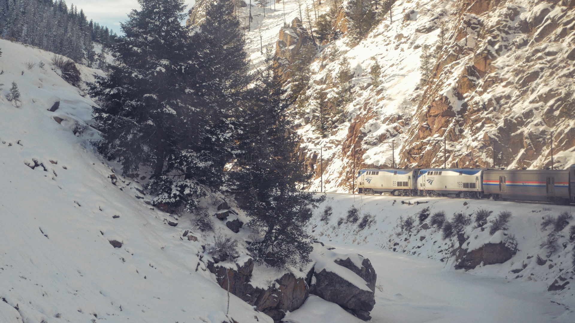
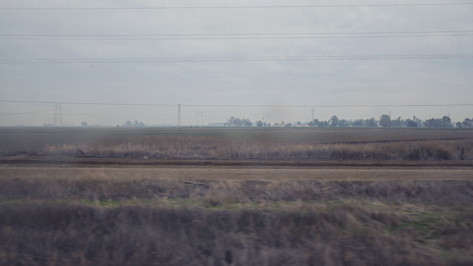
California Zephyr, 2020 Winter Break Trip
During the winter break between Dec. 2019 and Jan. 2020, I went on a great trip across the US: starting from Michigan, I went to Illinois, took a train (the California Zephyr) to California, then drove to Nevada, Utah, and in the end Arizona. This trip took us 18 days and we found great joy in it, especially in photography.
This is a reprinted travel journel about the California Zephyr from my friend that traveled with me, Junjie Luo. He wrote it in Chinese so it will also be in Chinese here.
这是一篇由当时同行的朋友撰写的加州和风号的游记,转载自微博@箫珏。
笔者在2019末体验了美铁加州和风号的全程。这篇文章主要以图片的形式记录这三天两夜的旅程,也会有一些介绍和个人的感想。为了保证观感,所有的链接攻略将放在结尾。全文图片较多,建议选择合适的网络环境阅读。
加州和风号简介&前言
California Zephyr,即加州和风号列车,是往返于伊利诺伊州芝加哥市和加利福尼亚州旧金山市近郊的长途旅客列车。目前的加州和风号为多家铁路公司的长途特快旅客列车合并联营而来,由美铁(Amtrak)经营。列车经由伊利诺伊州,爱荷华州,内布拉斯加州,科罗拉多州,犹他州,内华达州,和加利福尼亚州,贯穿美国中西部和西海岸地区,全程3924千米(2438英里),用时约52小时,是美铁旗下运行线路最长的城际列车之一[1]。
![加州和风号线路图[2]](/2020/05/18/california-zephyr-junjiel/Picture1.PNG) 加州和风号线路图[2]
加州和风号线路图[2]
列车穿越大平原,洛基山脉,科罗拉多河谷,内华达山脉等地,沿途风景优美壮丽[1],可以看到不同的景观,因此一直以来都是笔者非常想要体验的列车。但苦于没有合适的机会,一直未能成行。正巧今年(2019年)寒假没有回国的安排,就约了同学一同去加州玩,暂时逃离密西根州的严寒。假期的时间相对比较充足,我们决定选择不那么快节奏的交通方式,放弃了飞机,选择了长时间的火车。由于加州和风号的观光性质,车票会比较紧张,特别是卧铺车票。如果有乘坐的打算,建议尽早购票。由于秋季学期学业繁忙,我们在出行前一个月左右才确定了行程,并且很幸运的买到了最后一张Superliner Roomette(加州和风号的席位之一,将会在之后的行程中介绍)的票,得以踏上三天两夜的火车行程。
正文部分
2019年12月19日,我们正式踏上了行程。由于笔者在密西根州的安娜堡求学和居住,需要先乘坐列车从安娜堡前往芝加哥,再在芝加哥换乘加州和风号列车。为了保证行程的完整性,从安娜堡到芝加哥的旅程也会进行简单的介绍。
安娜堡到芝加哥
12月19日一大早,我们便来到了安娜堡车站,准备搭乘早上7点20分发车的列车前往芝加哥。清晨的安娜堡站泛着一层粉色的朝霞,很是好看。安娜堡车站很小,只有一个站台一条轨道,是美国铁路客运衰落的环境下很多车站的现状。加州和风号在这样的环境中能够留存,可以说是非常可贵了。
 清晨的安娜堡车站
来到车站后不久,我们便得到了一个不幸的消息,前往芝加哥的列车晚点未定。笔者拿出手机查了一下这趟车,发现列车尚未从始发站发出。一时间笔者和朋友陷入了恐慌,甚至打算实在等不到车就租车开去芝加哥。好在晚点一个半小时之后,列车终于到达了安娜堡站。由于预留了较为充分的换乘时间,后续行程未受较大影响。在此也提醒大家出行留够时间,做好备用方案。
 列车晚点一个半小时进入安娜堡站
从安娜堡前往芝加哥全程四个半小时左右。由于这趟列车不是本次行程的重点,在此就不做详细介绍了,不过还是放一些车内的图片,方便大家对美铁有一个大致的印象。如果有兴趣了解的话可以搜索列车名Wolverine了解(这趟车似乎没有通用的中文译名,直译的话是“狼獾”之意)。
 普通车车内,自由席,由于早起补觉,并没有去拍商务车内饰
 座位间距整体比较宽,窗户很长,没有面壁
 刚下过雪,配上阳光,景色不错,可惜玻璃比较脏
 空间很大的无障碍厕所
由于列车晚点时间较长,美铁的列车员给每位乘客发了一小袋零食和水。笔者也从列车员口中大致了解到晚点原因是电脑故障导致了车厢的电器设备无法启动,灯和空调都无法运行。
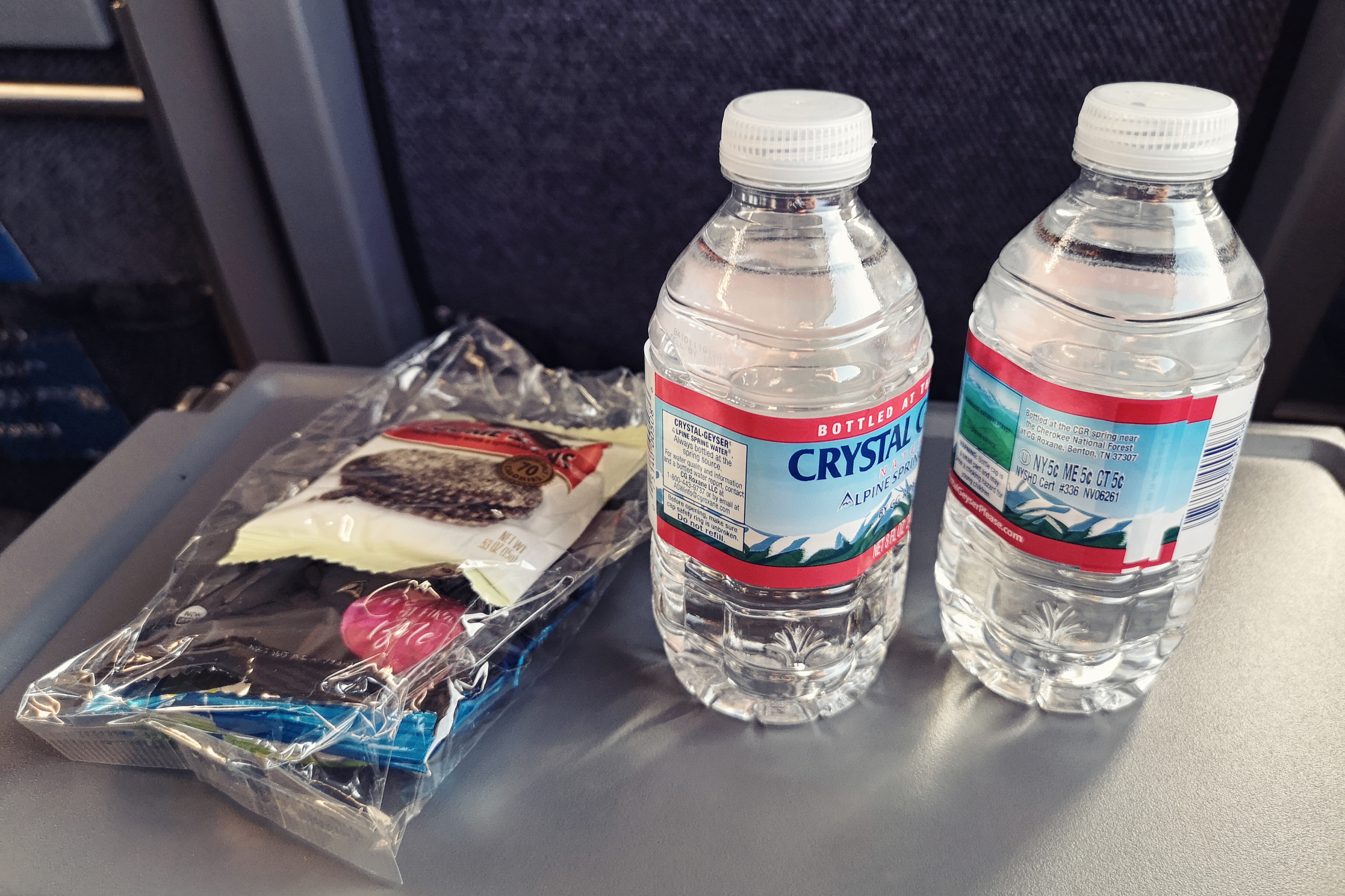 赠送的零食和水
 全程最高时速(换算为公制单位为176 km/h,这个速度并不能持续很久
虽然列车尽力追回晚点,但由于之前晚点太久,时刻表被打乱,在途中又避让了几列货车,最终列车晚点了两小时左右,在当地时间下午一点左右到达芝加哥车站。此时离加州和风号发车的时间仅剩下一个小时了,因此,我们不得不放弃了在芝加哥吃午饭的计划。
 列车到达芝加哥联合车站
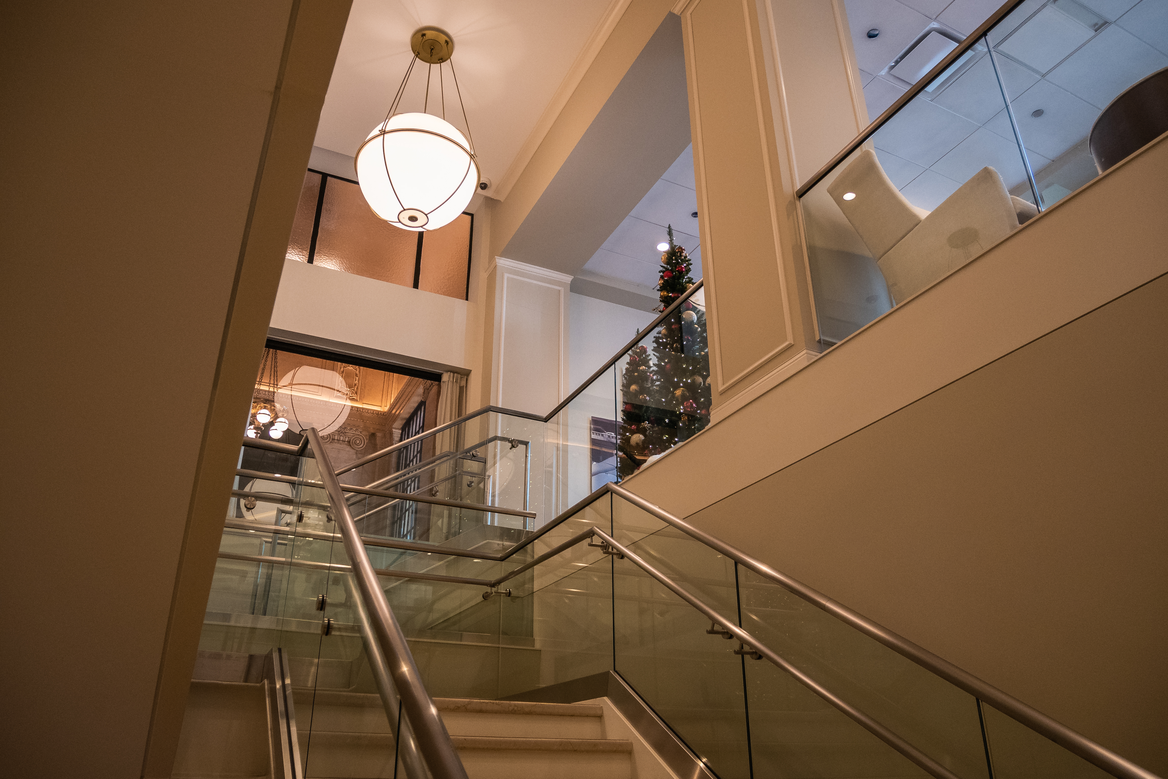
虽然时间比较紧迫,但我们还是抽空在联合车站里逛了一下。整个联合车站保留着上世纪的建筑,配上圣诞节的装饰,很是好看。
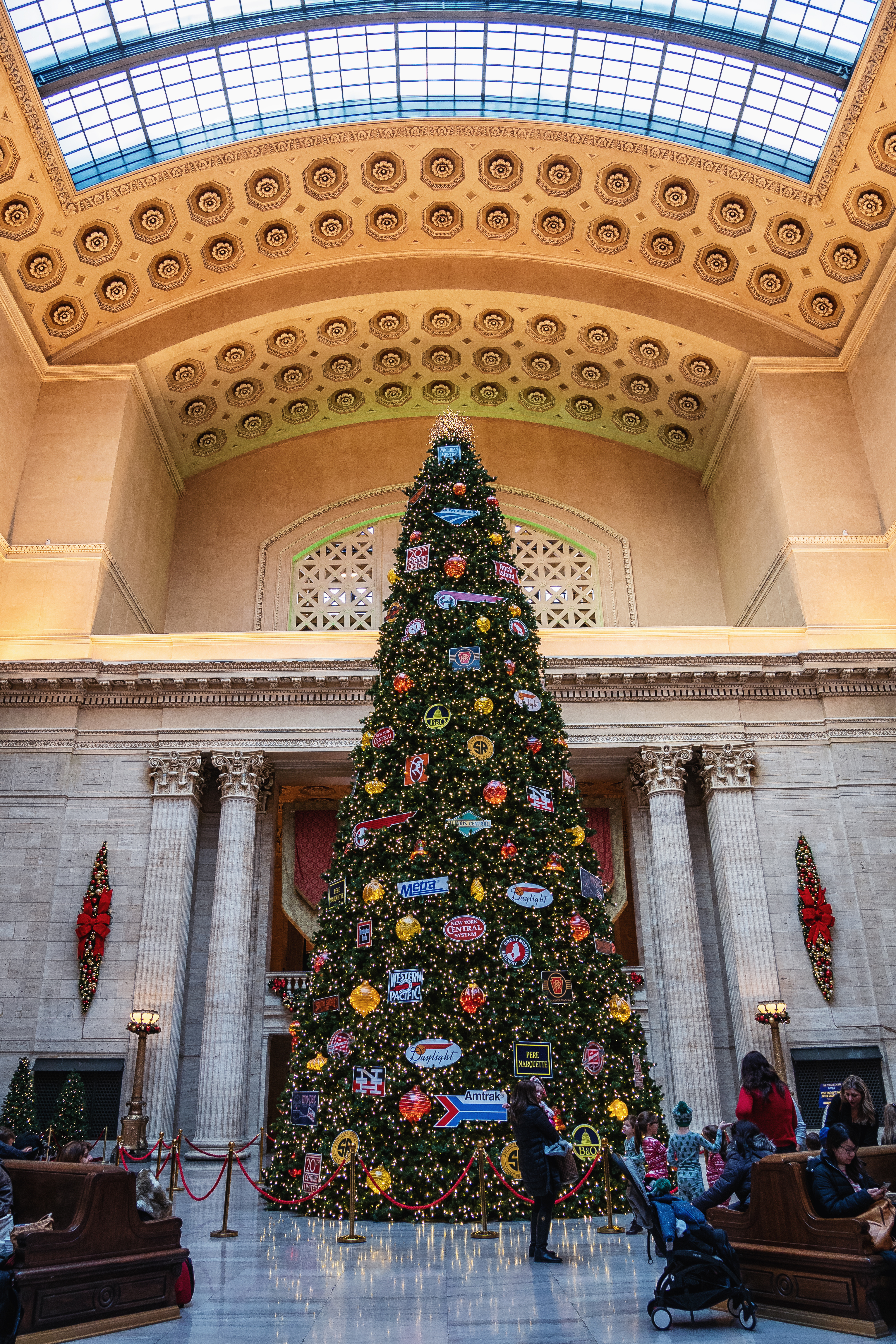 联合车站内的圣诞树
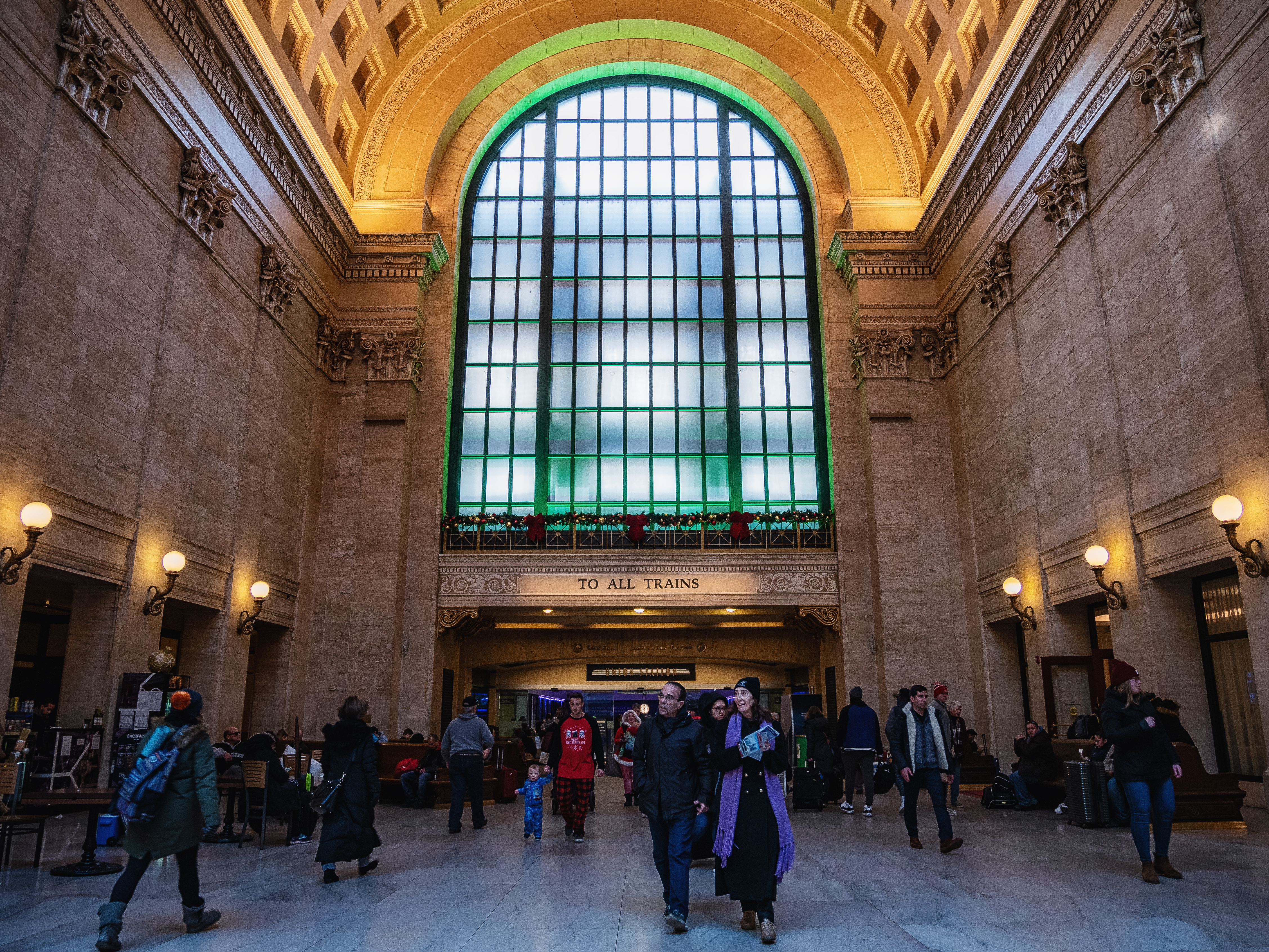 联合车站大厅
作为购买了卧铺车票的乘客,我们可以免费使用美铁的 Metropolitan Lounge,类似于商务候车室。可惜之前列车晚点,我们没有太多的时间来体验,只是进去转了一圈,没有拍太多照片。
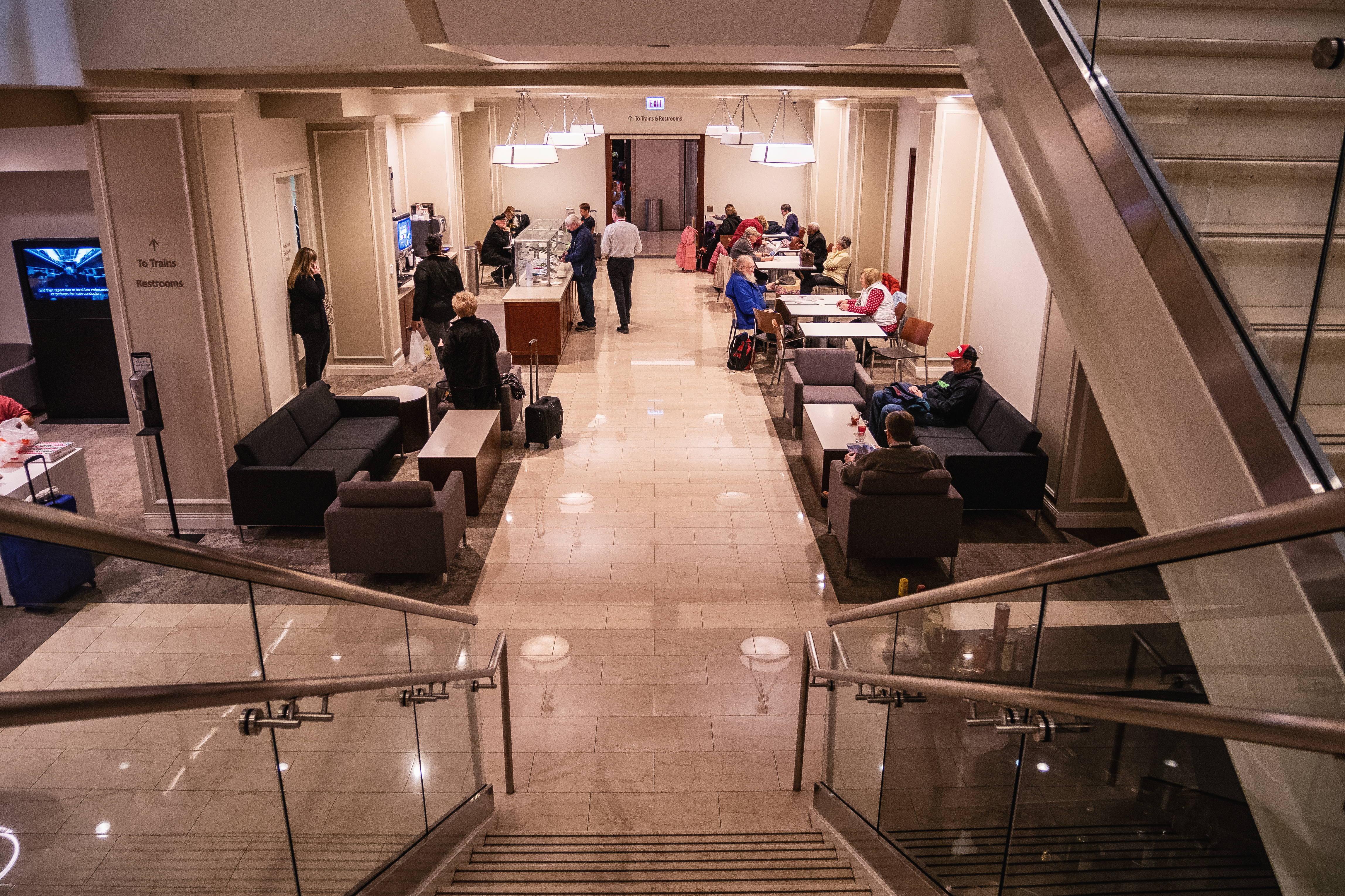 从楼梯上望向一楼。人比较多。中间左侧的柜台提供自助沙拉饮料,但也仅限于此
 从楼梯上望向二楼
还没在候车室转多久,我们便收到了检票上车的通知。
登车以及车辆简介
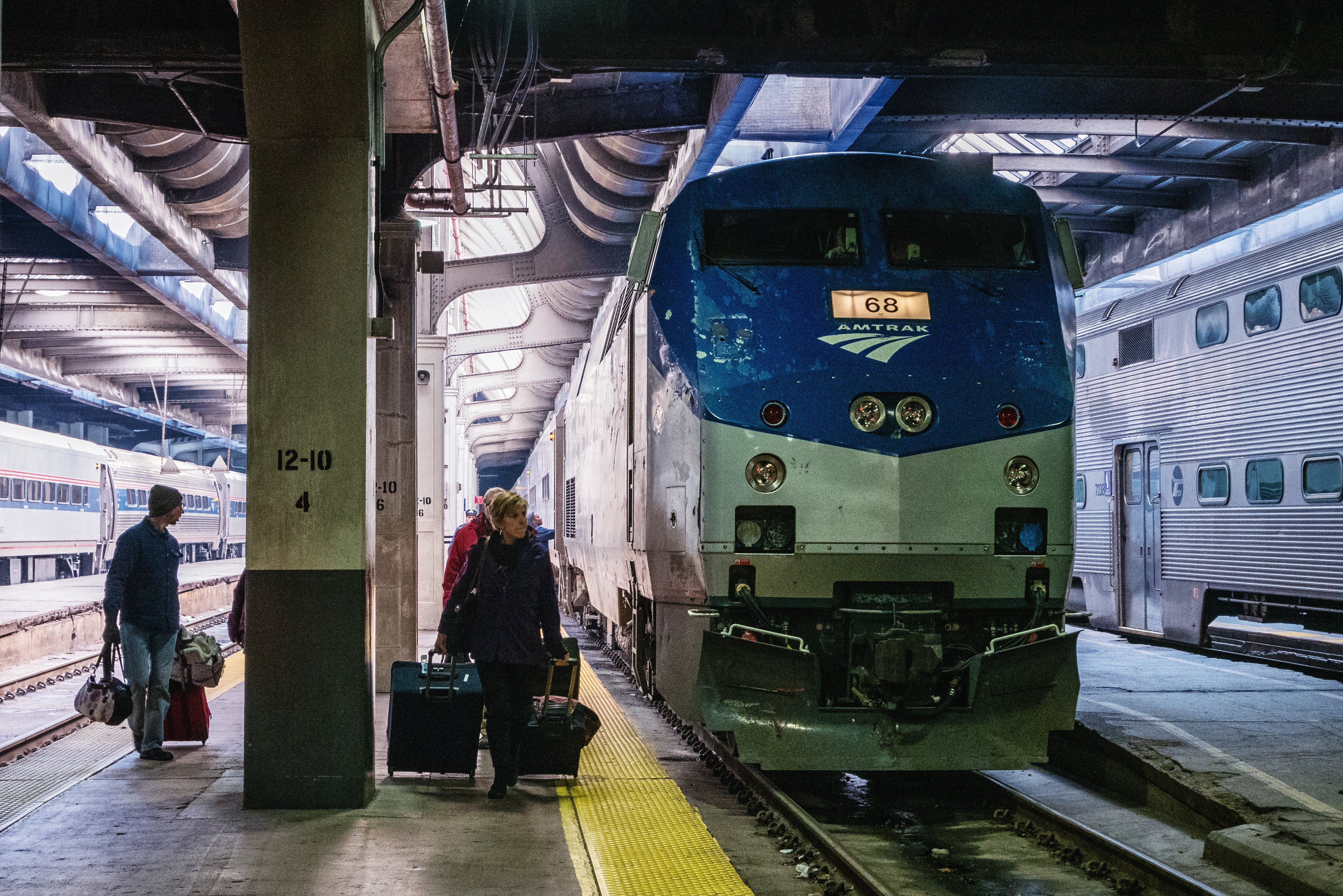
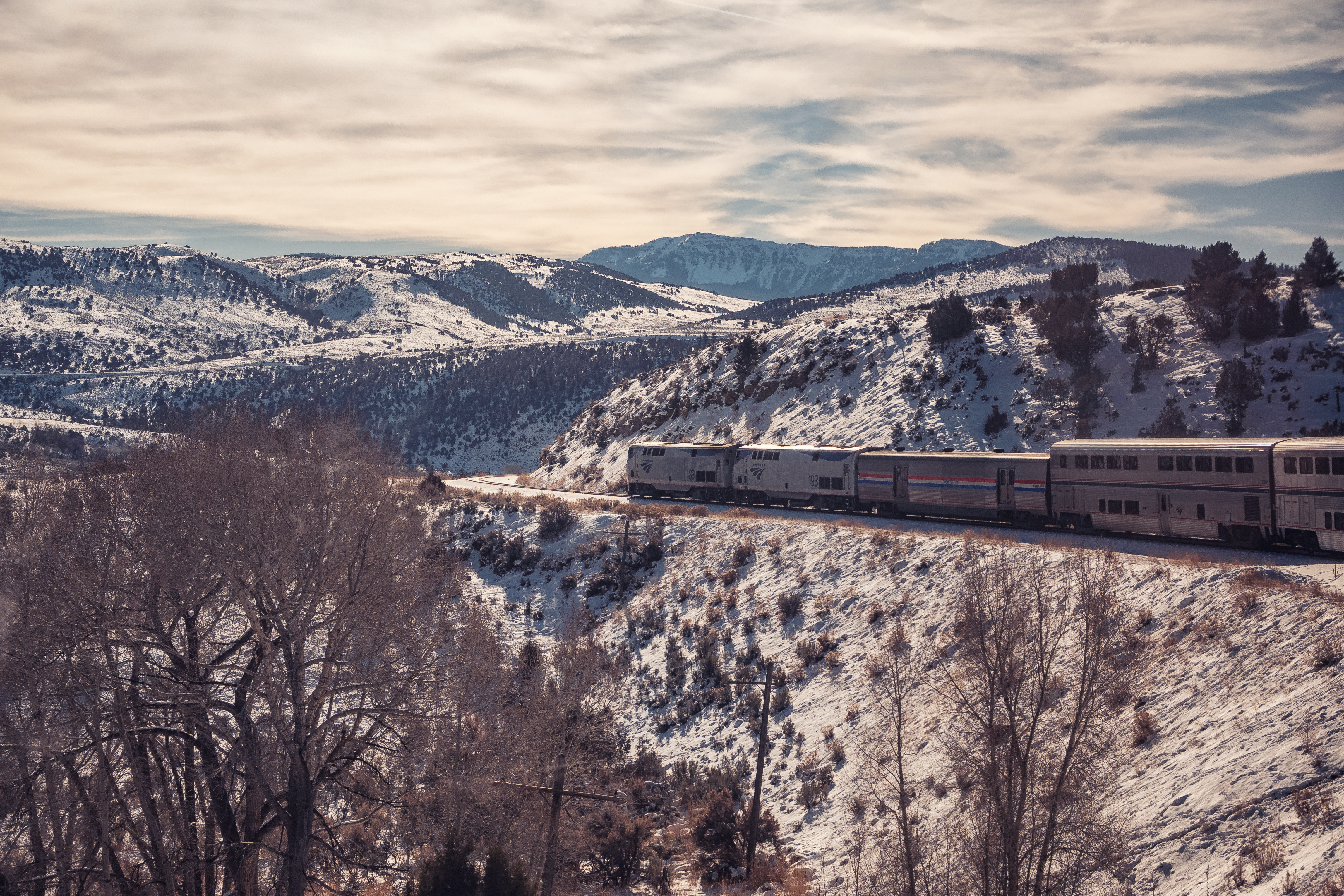
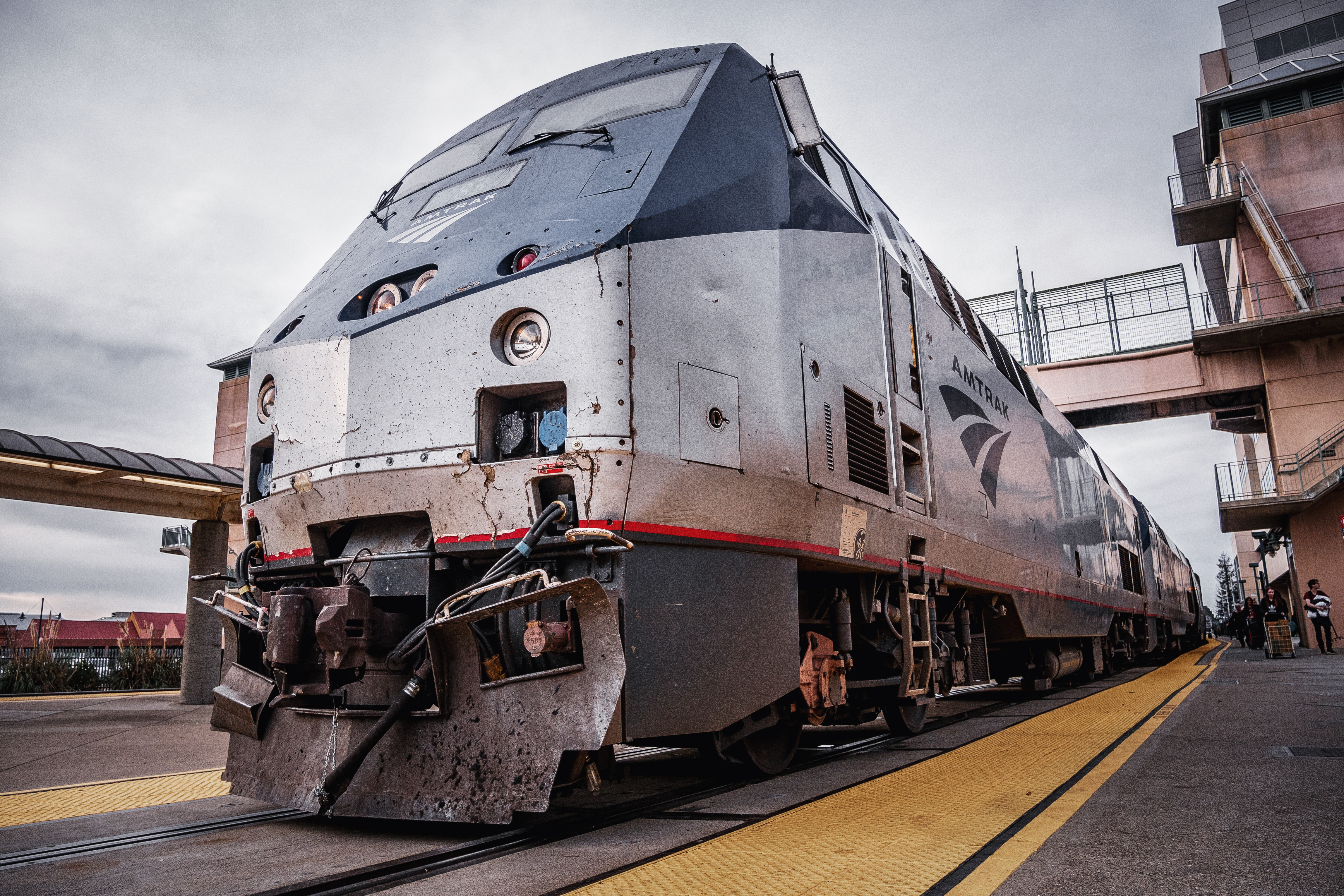
穿过专门的通道,走上站台,我们终于见到了本次行程的主角,加州和风号。
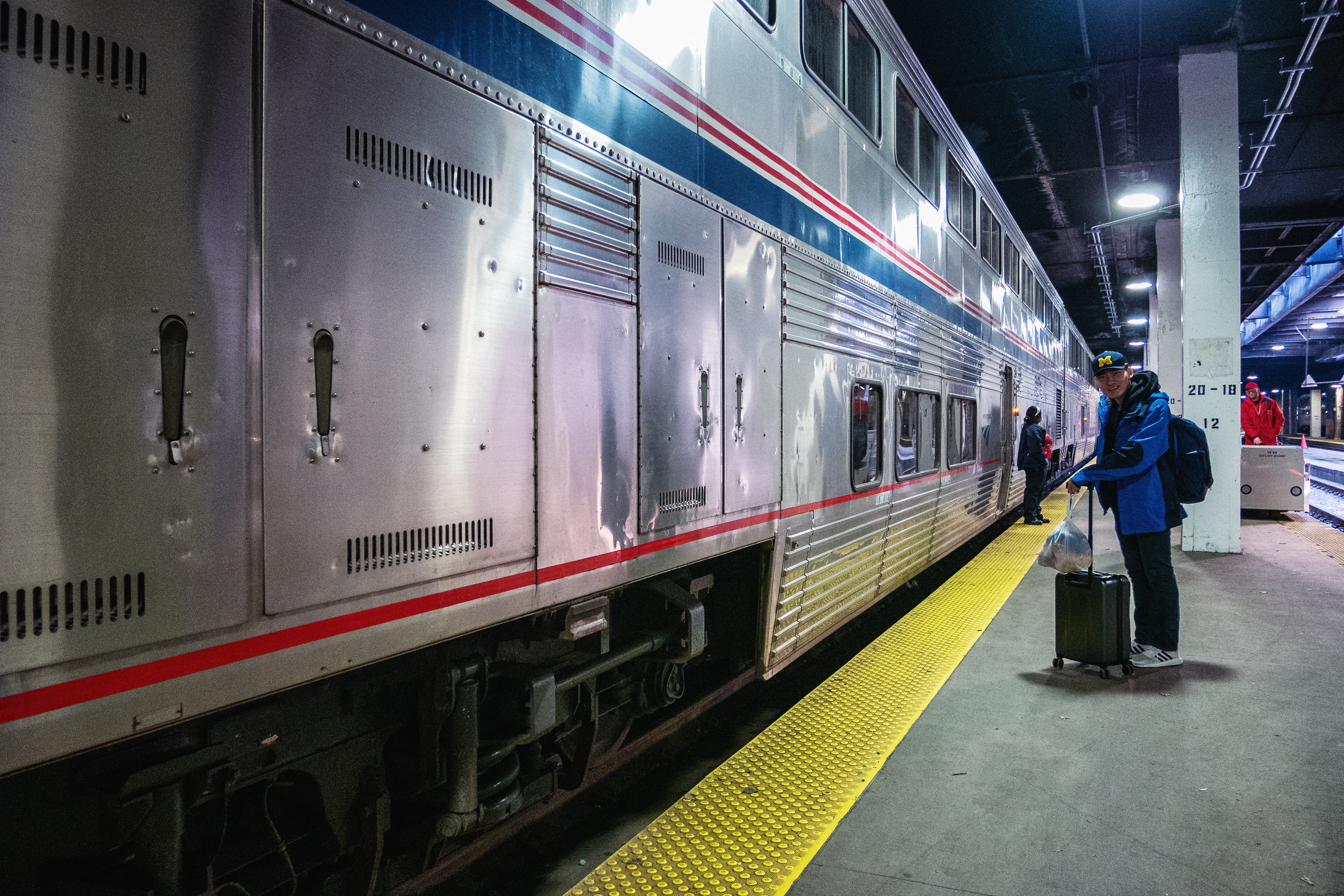 停靠在站台的加州和风号,双层的车厢非常高大
在此简单讲一下列车的编组,列车的编组并非完全固定,但形式上大致上遵循两台P42DC柴油机车+1节行李车+4节双层卧铺车+1节餐车+1节观景车+3节坐席车。(其中可能包含坐席行李,坐席餐吧合造车)[1] 在此也放一张之前在芝加哥拍车时拍到的加州和风号的照片,希望可以对编组有一个更加直观的感觉。
 从联合车站出发的加州和风号,注意机后第七位的观景车顶部有窗户,较好辨认
我们所乘坐的是机后第四位的双层卧铺车。在开始介绍行程之前,笔者打算先介绍双层卧铺车Superliner车内的一些设施。如果对双层卧铺车已经比较了解,可以直接跳到章节2.3阅读行程部分。
双层卧铺车厢Superliner的内部结构图如下
![车厢内部结构[3]](/2020/05/18/california-zephyr-junjiel/amtrak-diagram-superliner-sleeper.jpg) 车厢内部结构[3]
车厢内部结构[3]
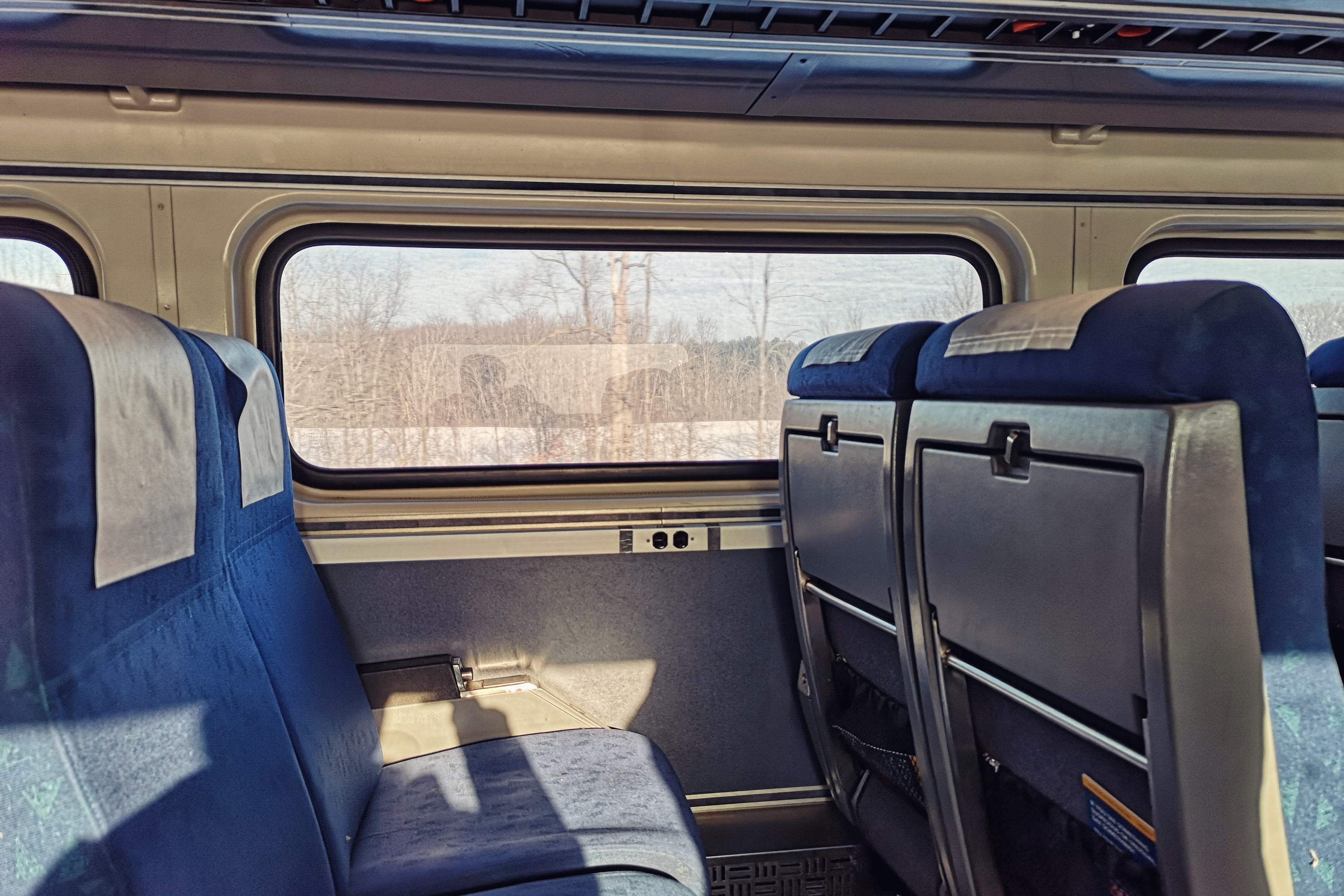
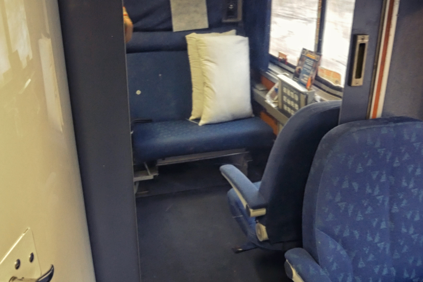
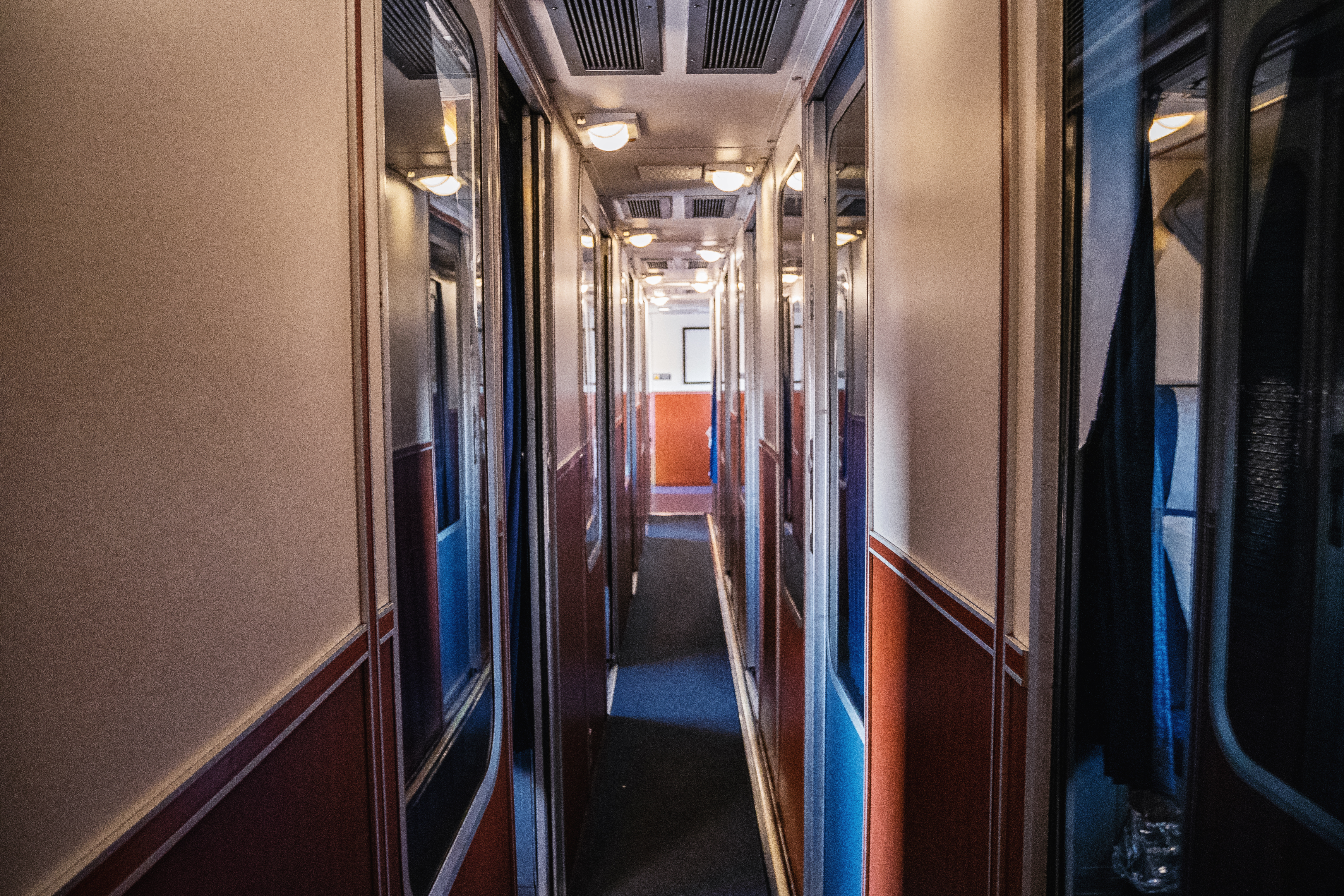
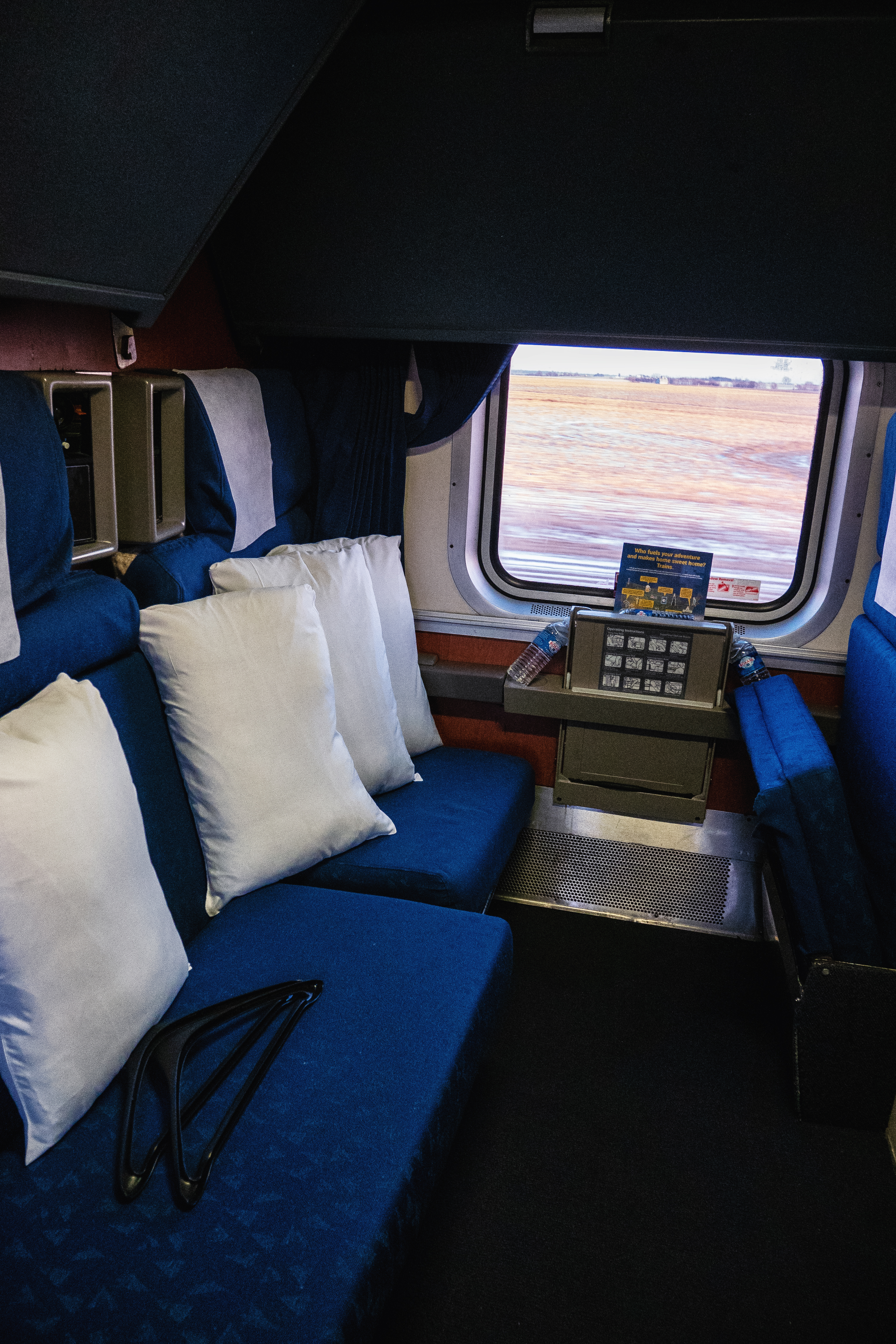
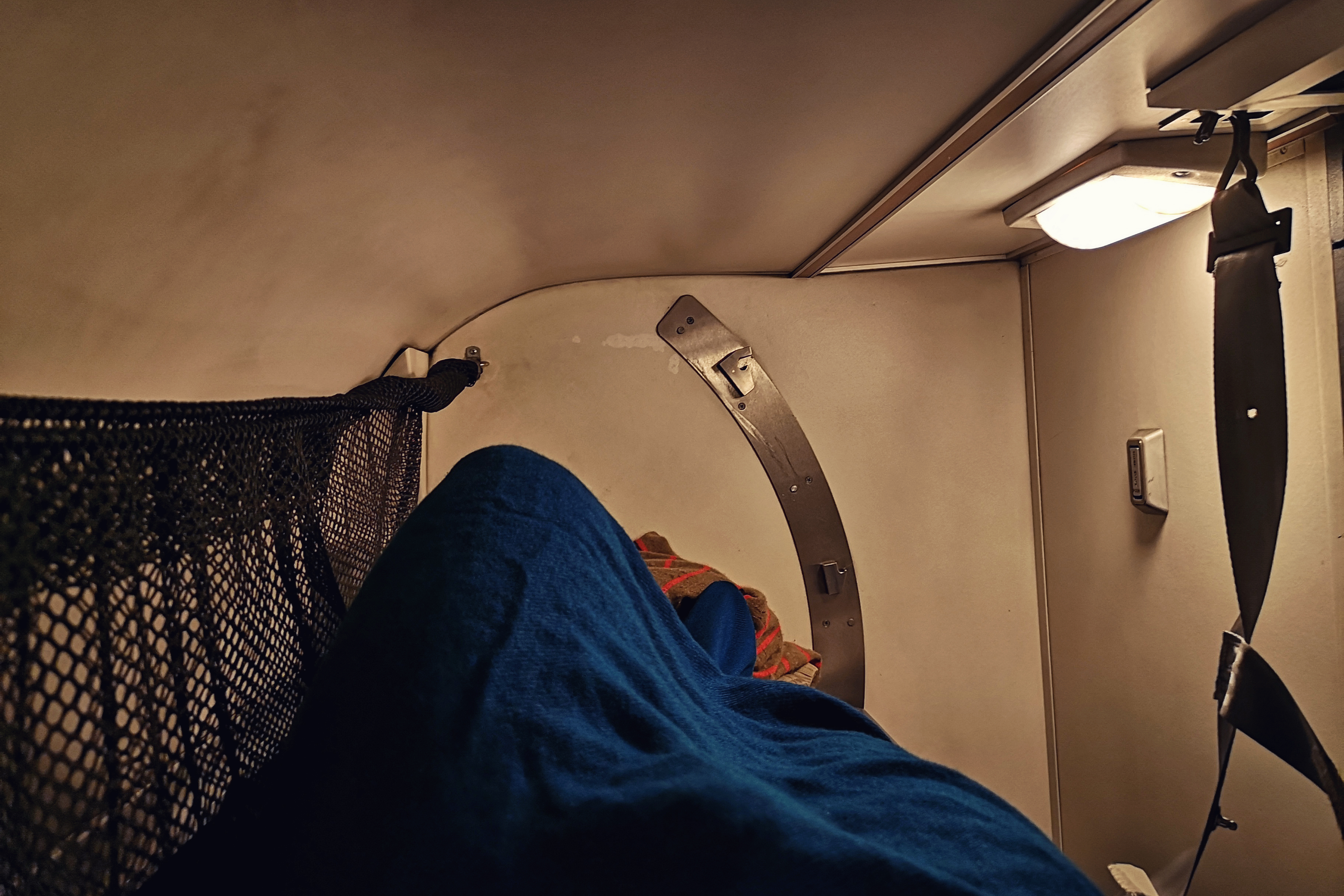
不同车厢的连接通道和大多数房间位于车厢上层。整个上层大概有一半空间都是我们所乘坐的狭小的双人间(10间),叫做Superliner Roomette。
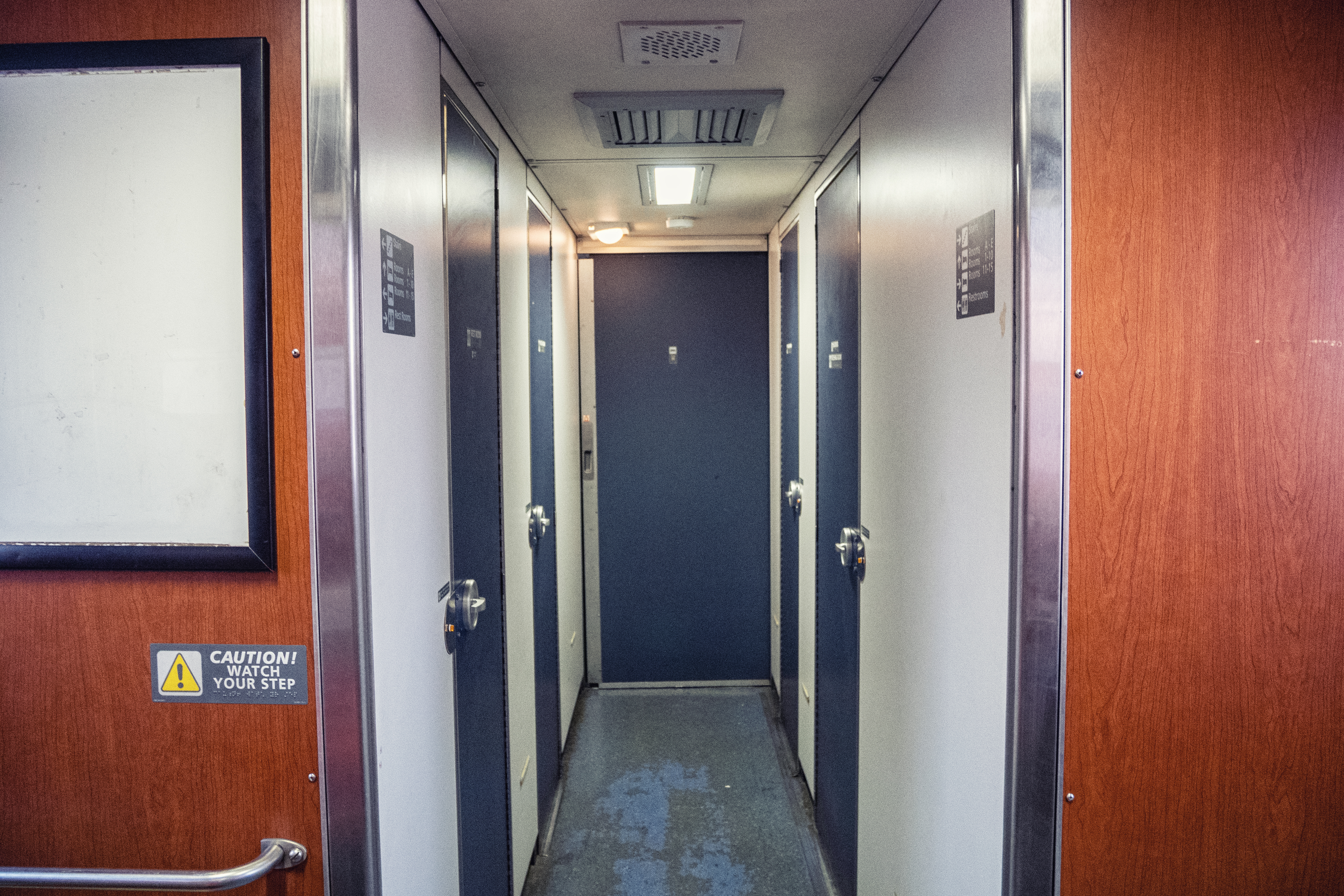 通道两侧都是小的双人间
Superliner Roomette这个席位的房间包含上下两张纵向的床铺,其中上铺可向上翻起,下铺由两张可拼合的椅子组成。由于自己的房间放了很多东西,所以部分图片借用了隔壁相同配置的空房间拍摄。(当然卧铺车票是全部售罄的,向列车员确认了,隔壁房间只是暂时空着)
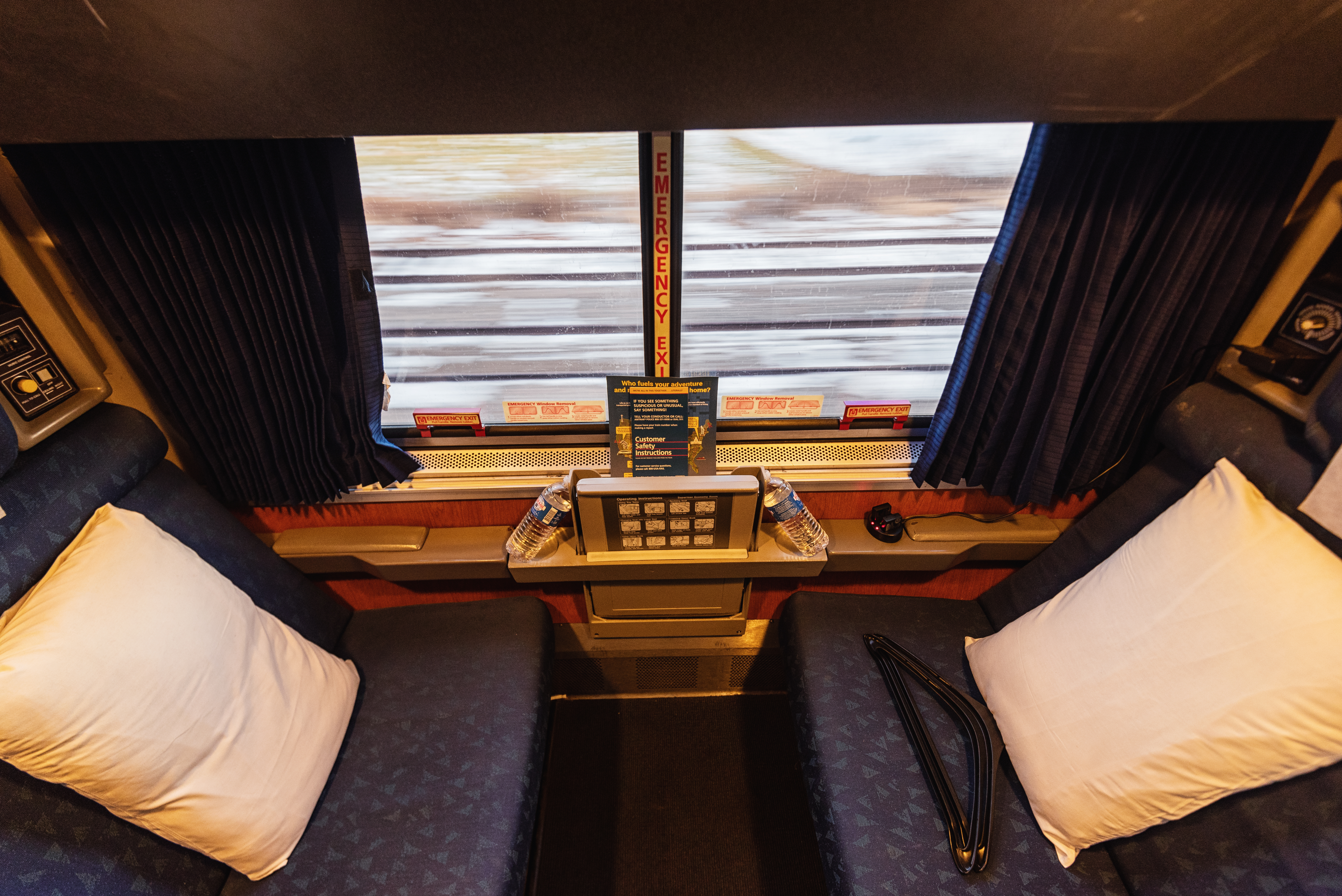 Superliner Roomette的整体概况,空间是比较狭小的
 坐在一侧的椅子上看向对面的视角
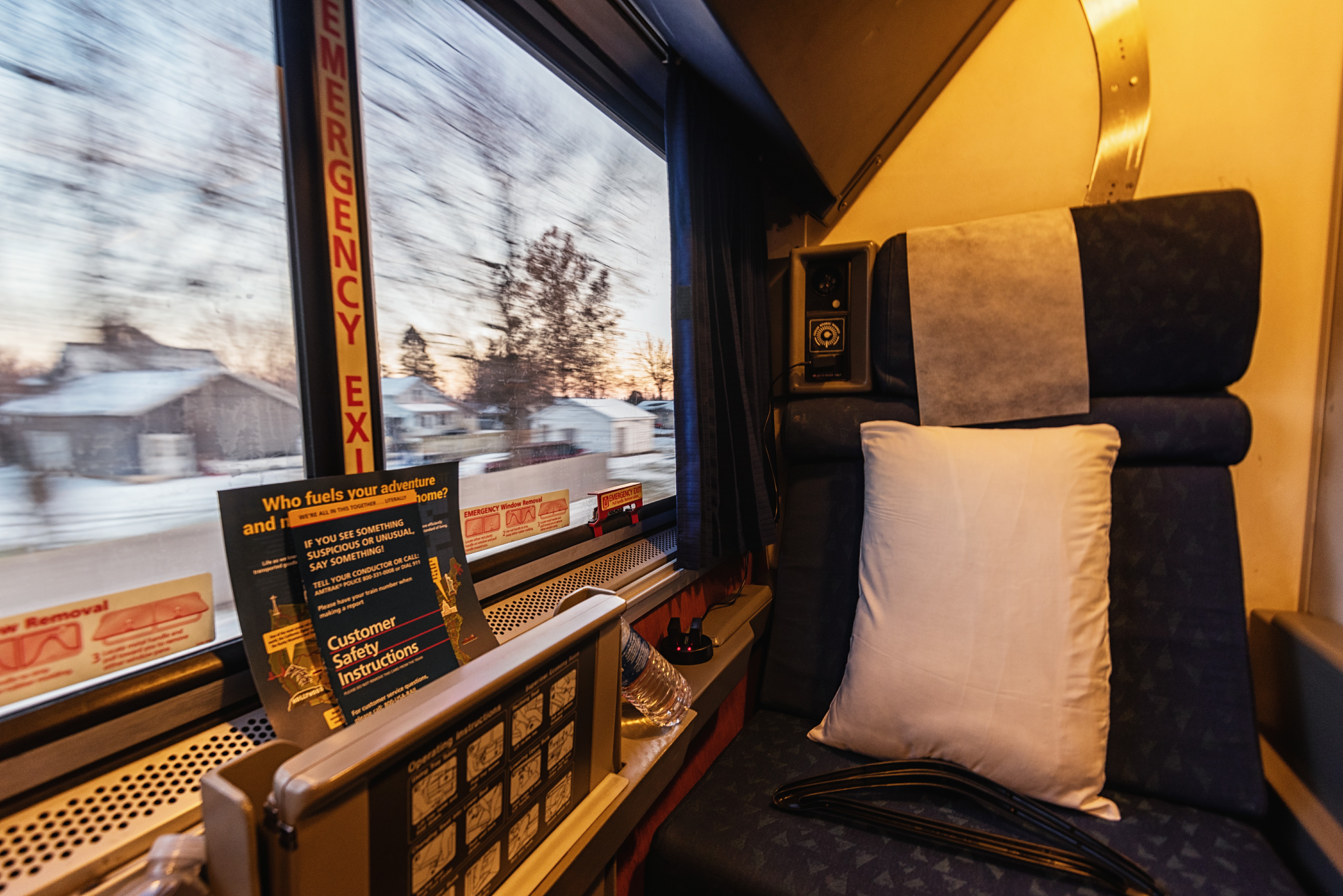
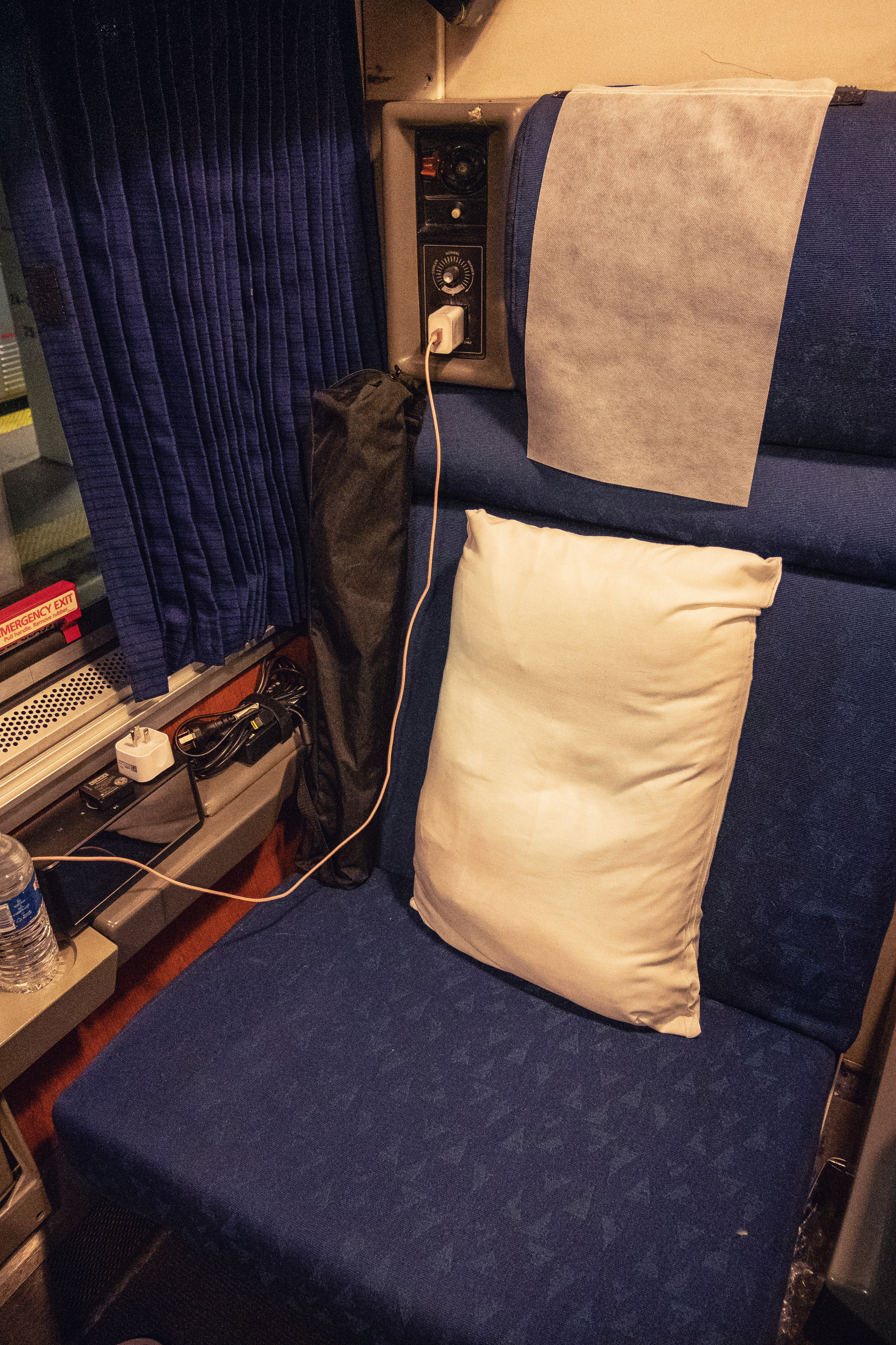
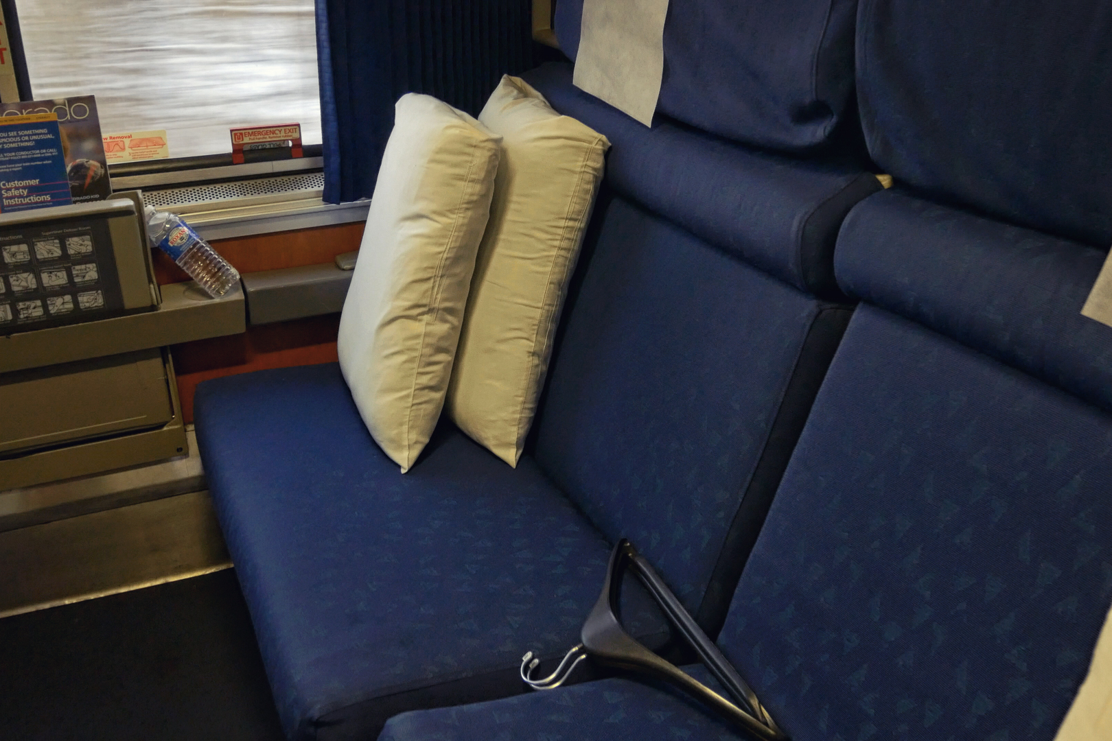
虽然房间内的空间不大,但是座椅比较宽,还是很舒服的。座椅的扶手上可以放下挺多东西。座椅边上有阅读灯的开关,空调温度调节装置和插座。注意整个房间只有这一个插座,如果设备比较多的话建议携带插线板或者把充电宝充满电。
 座椅的细节
座椅的细节
另一侧的座椅,从上至下是阅读灯,没有搞清楚怎么用的音乐控制,呼叫按钮和房间内的整体灯光控制。
其他的一些部件和细节展示,部分图片为视频截图,存在模糊,还请见谅。
 上铺有独立的阅读灯
车门可以从内部锁上,同时还提供一个可以拉上的帘子,私密性不错,但可惜的是并不能从外侧锁上,所以在去较远的地方的时候还是建议携带上贵重物品。
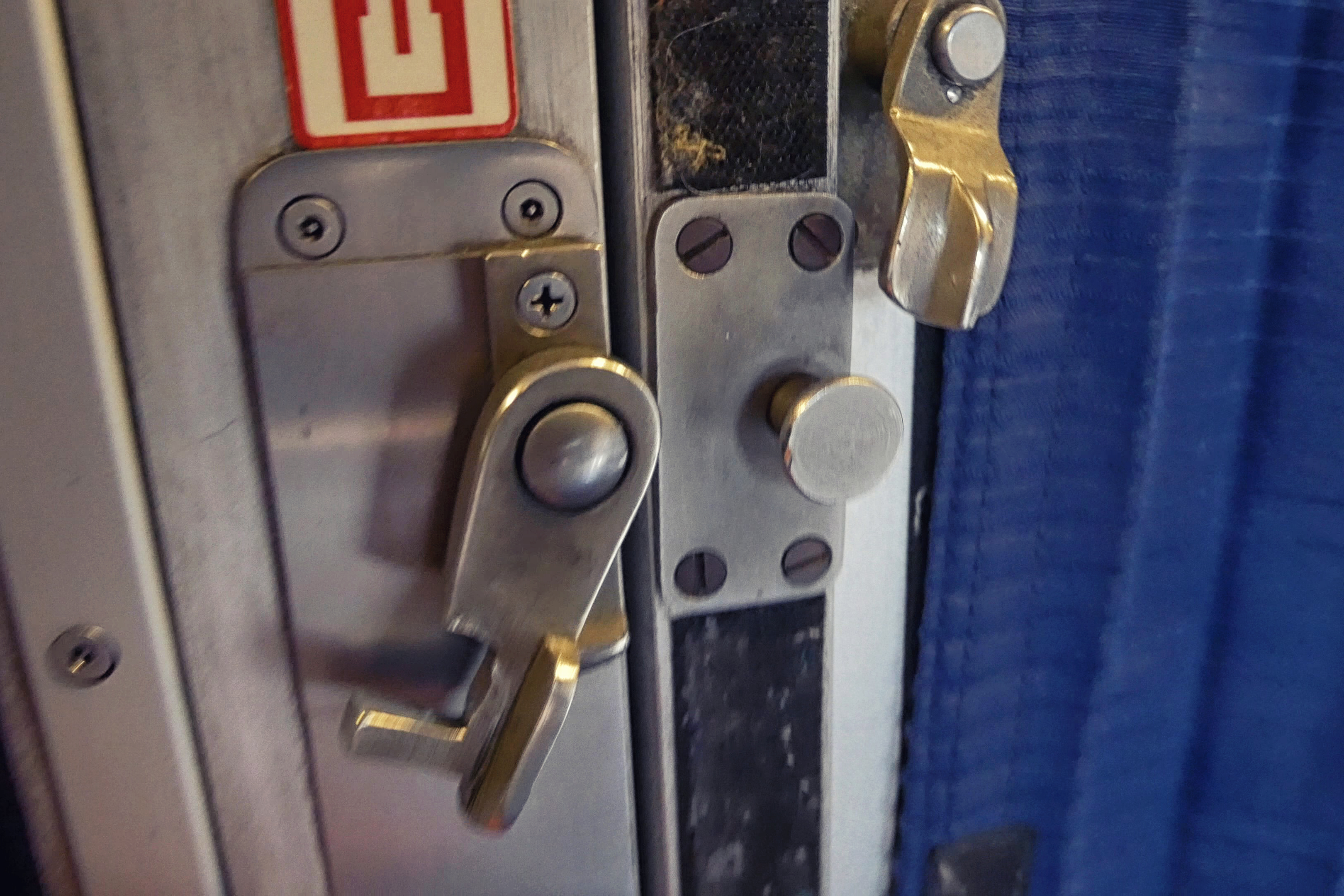 车门细节
车门细节
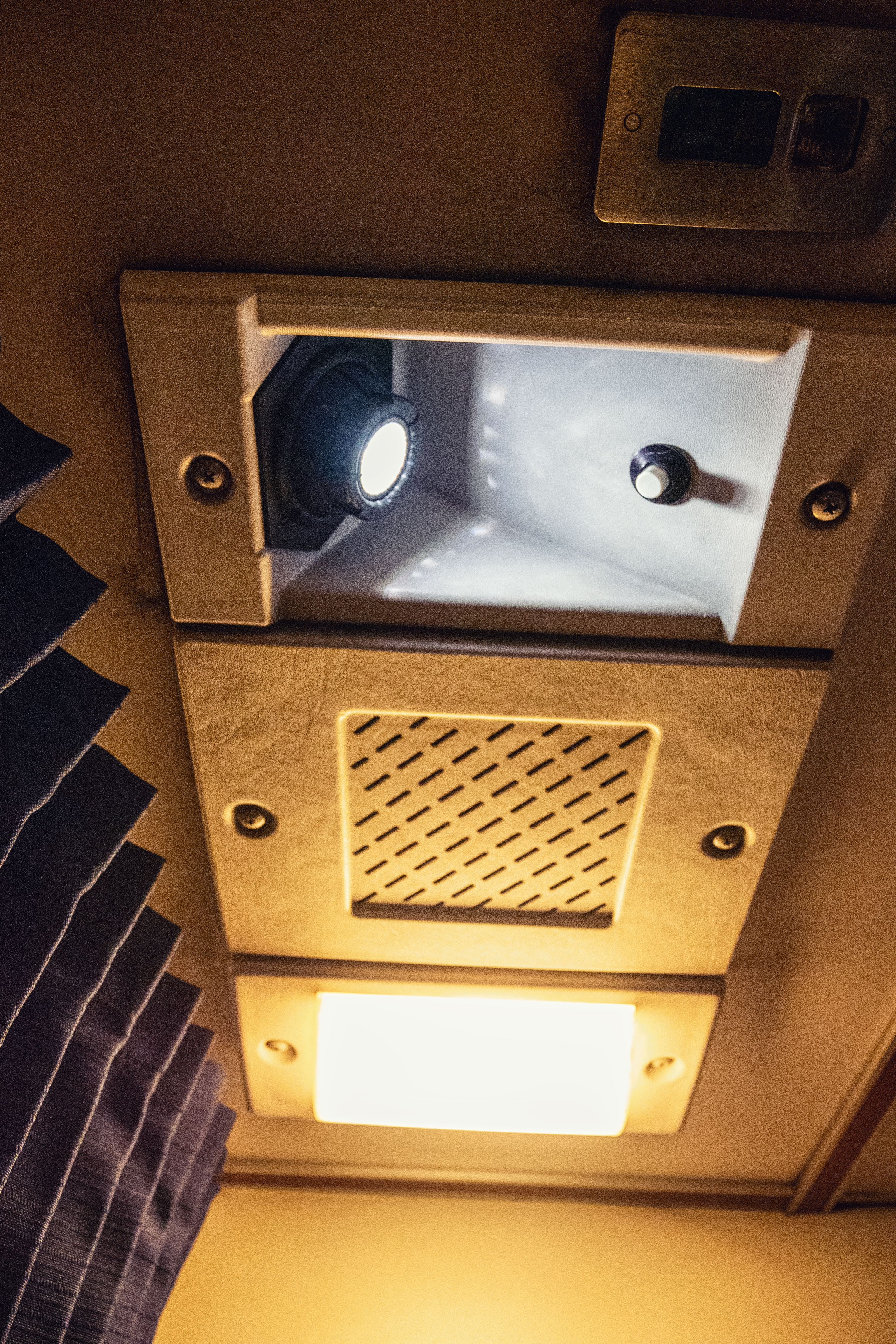
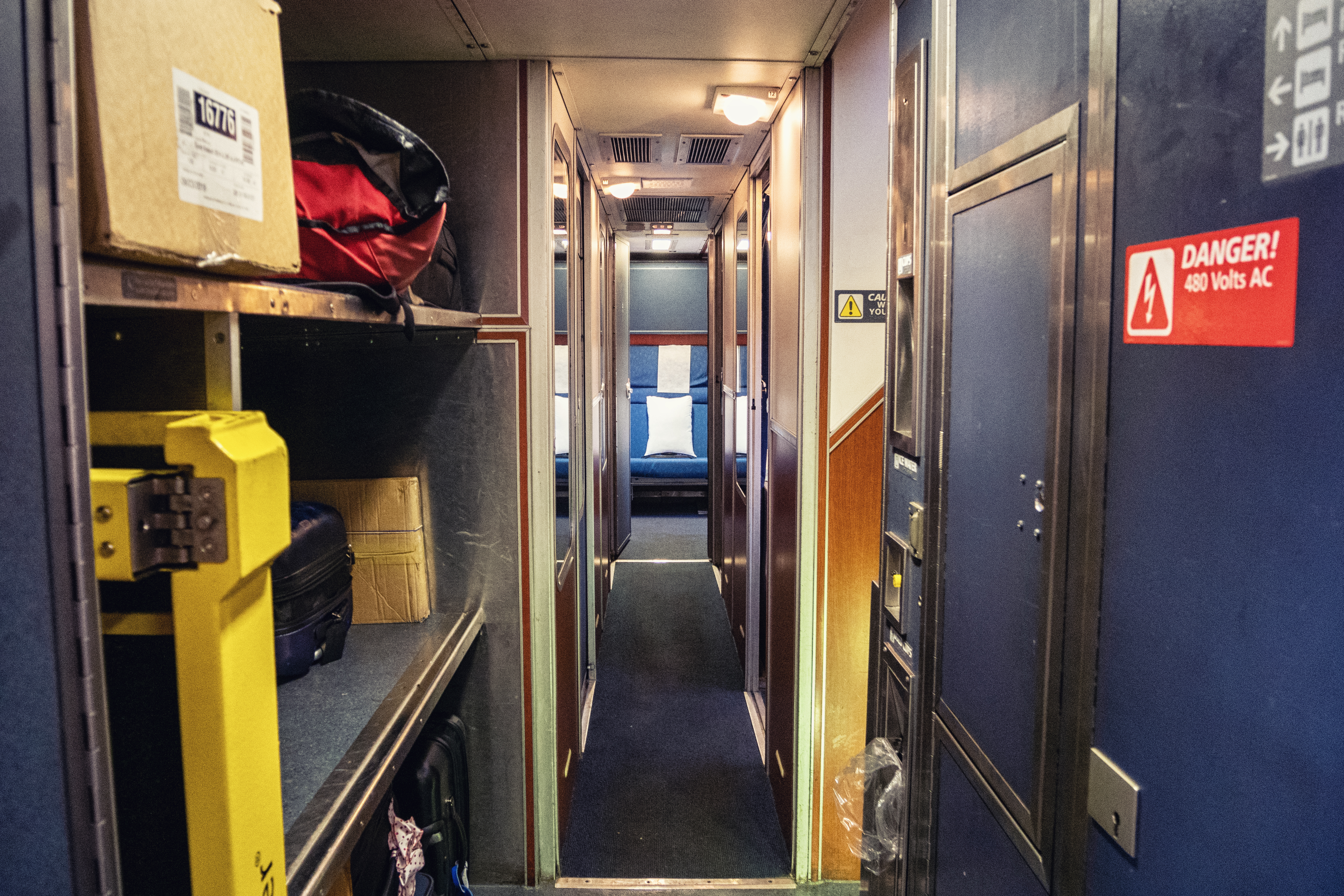
逛完了自己的房间,就去车厢其他地方走走。车厢上层中部有一个厕所,通往下层的楼梯,咖啡机,以及可以接取冰水的饮水机。
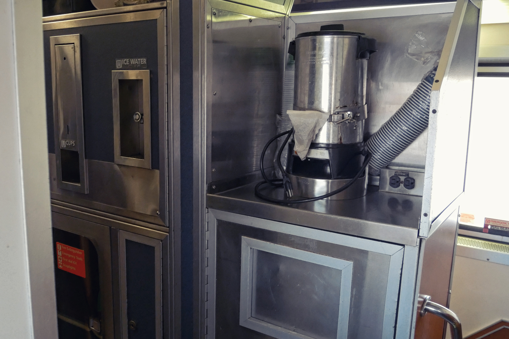 上层中部细节
上层的另一侧是较大的双人间Superliner Bedroom,两间Superliner Bedroom中间有门,可以组合成套间(Suite)。笔者进入了其中一间空着的房间,拍摄了一些照片。和我们住的小房间相比,大房间内的空间大很多。其中有两张横向的卧铺,一张椅子,一个卫生间,一个洗漱台。这样的配置显然比我们的小房间豪华不少,当然价格也会高不少。顺带一提这个双人间的下铺是可以睡两个人的,如果实在有需要的话可以变成三人间。
 床铺
床铺
 椅子和连通隔壁房间的门(视频截图,模糊请谅)
 自带卫生间
自带卫生间
 自带洗漱台(视频截图,模糊请谅)
然后去往车厢下层。车厢内的楼梯比较狭窄,也比较抖,对年龄较大的人有一些不太友好。
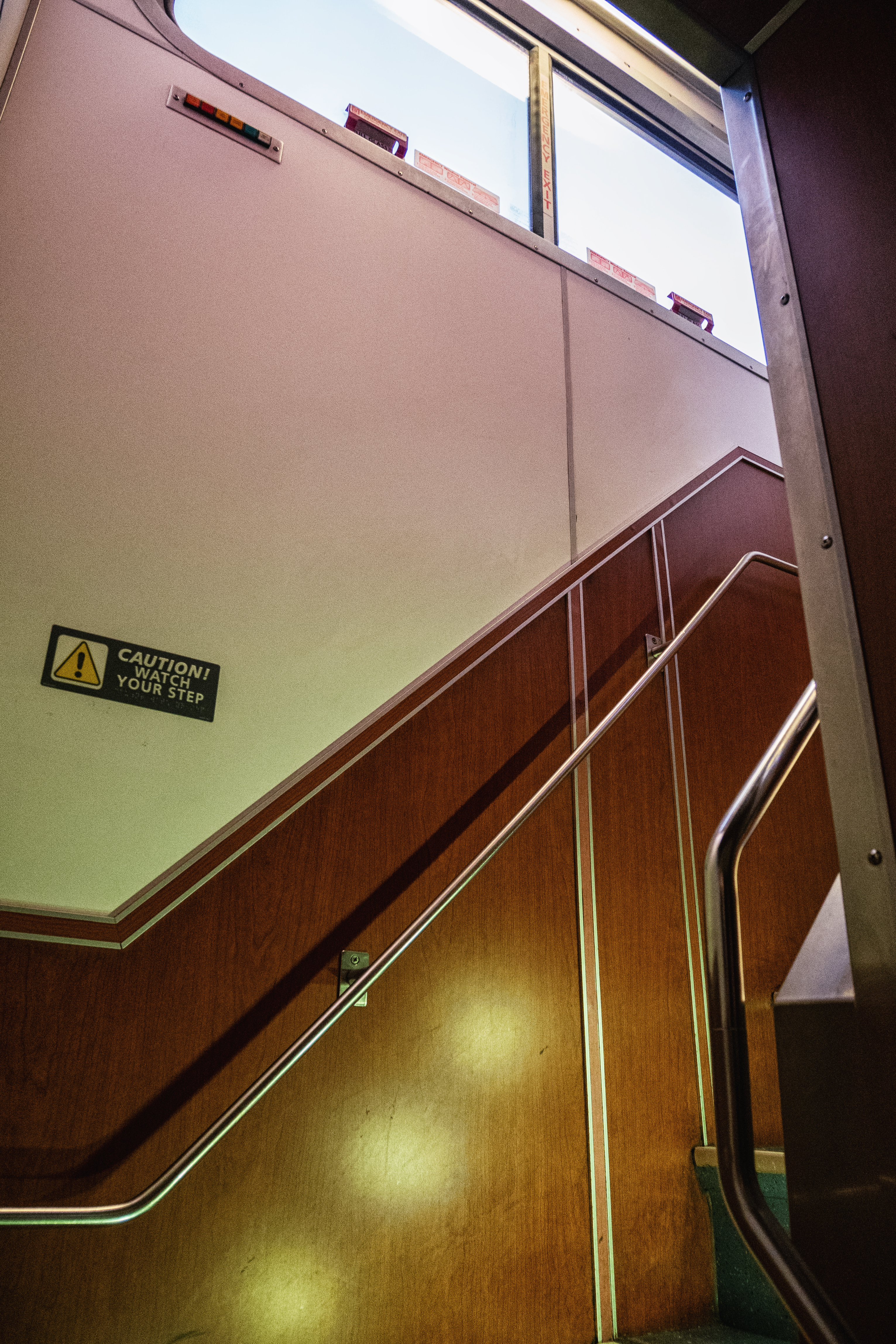 楼梯
楼梯
走下楼梯,就可以看到大件行李存放处。因为房间空间并不是很大,所以除了贵重物品之外的行李就存放在这里。
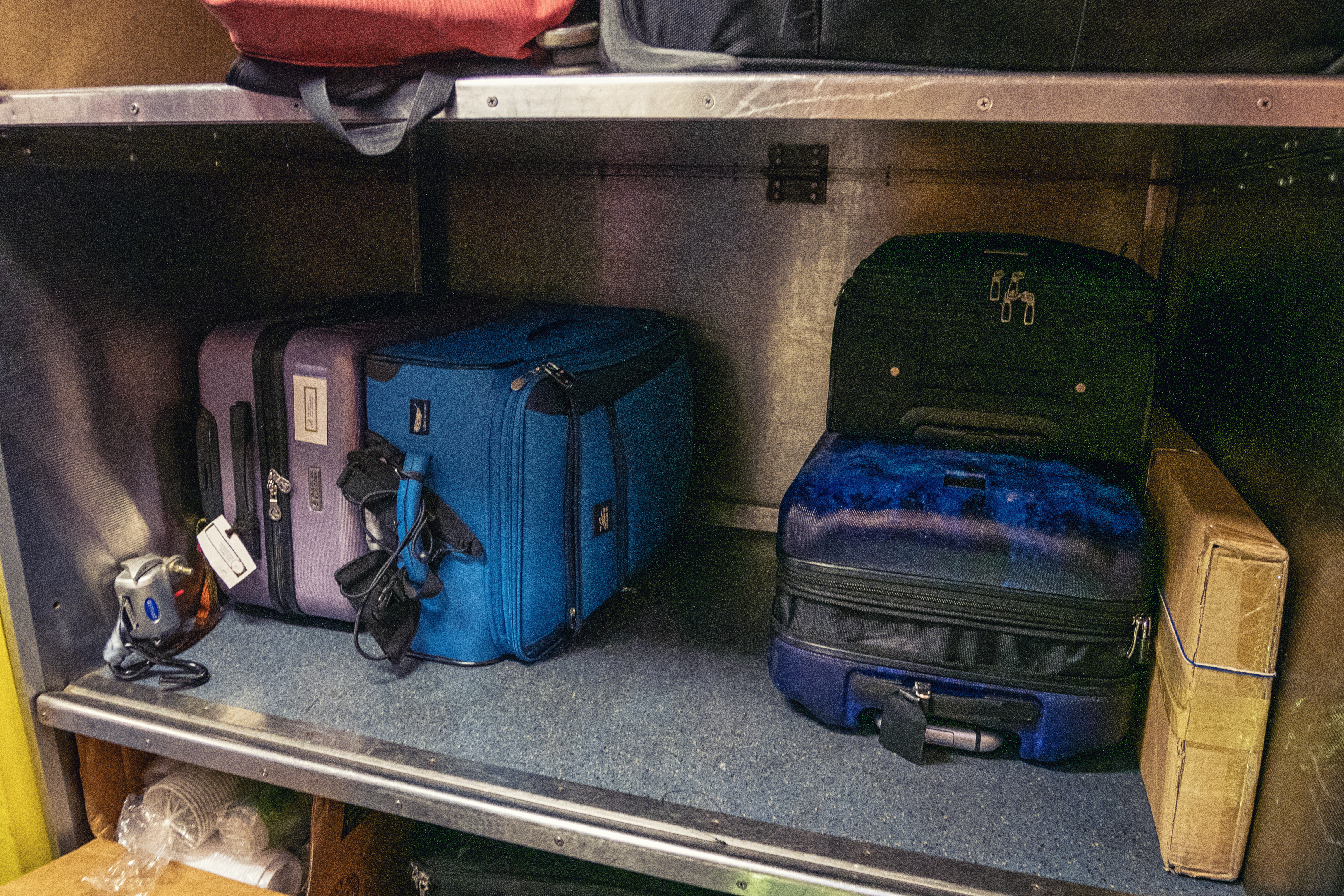 行李存放处
行李存放处
行李存放处的旁边就是车门。注意那个黄色的小板凳,是美铁标配的站台补偿器( ̄▽ ̄)*
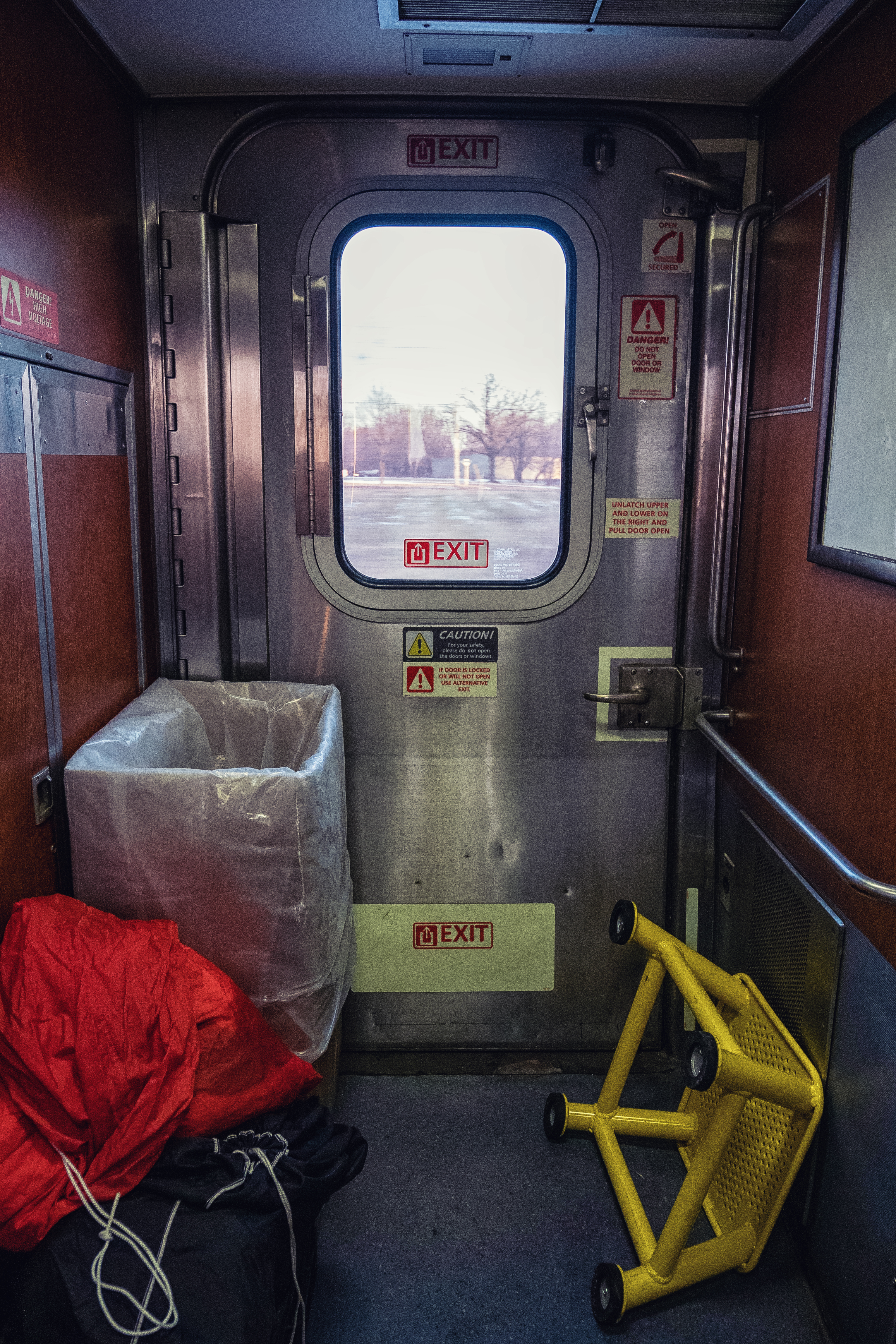 车门附近
车门附近
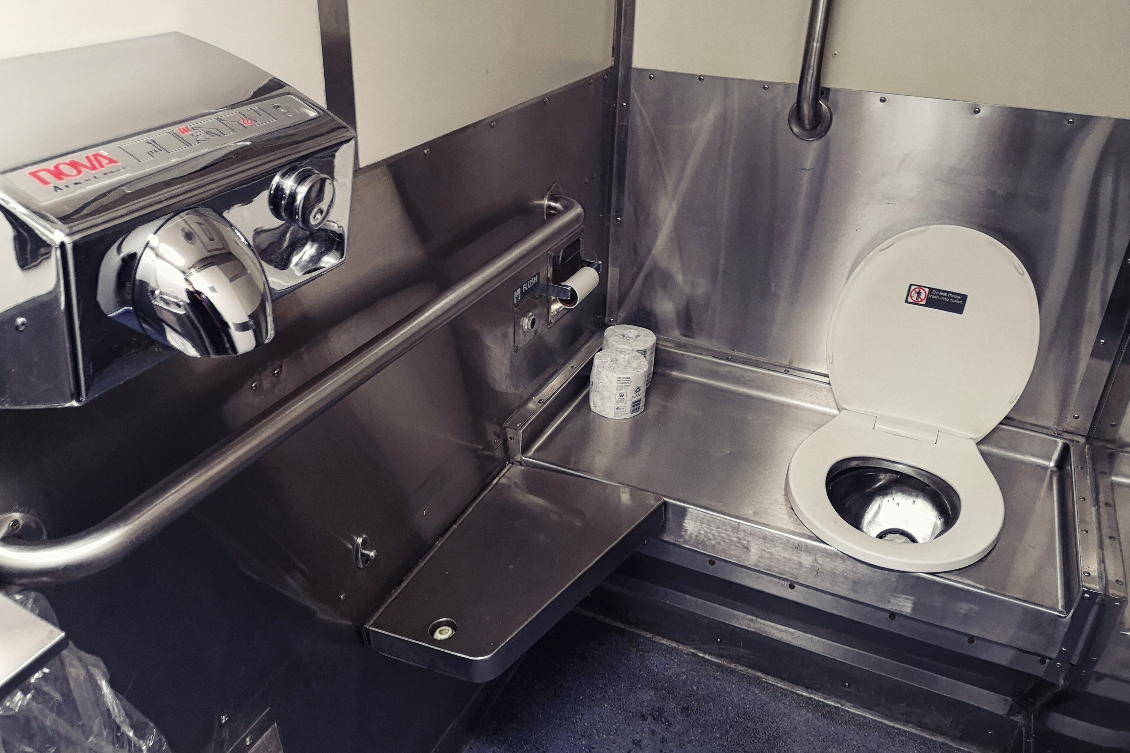
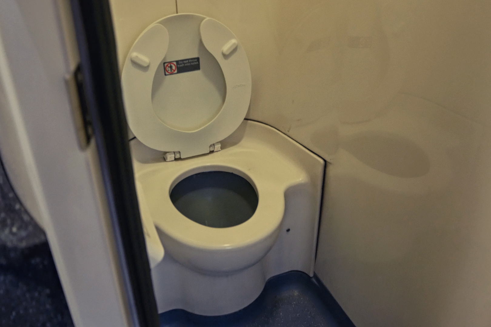
下层的一侧有4间小的双人间和一间家庭套间,另一侧有三个卫生间,一个浴室和一间无障碍房间。
 下层的一侧,卫生间和尽头的无障碍房间
 下层的另一侧,尽头是家庭套间
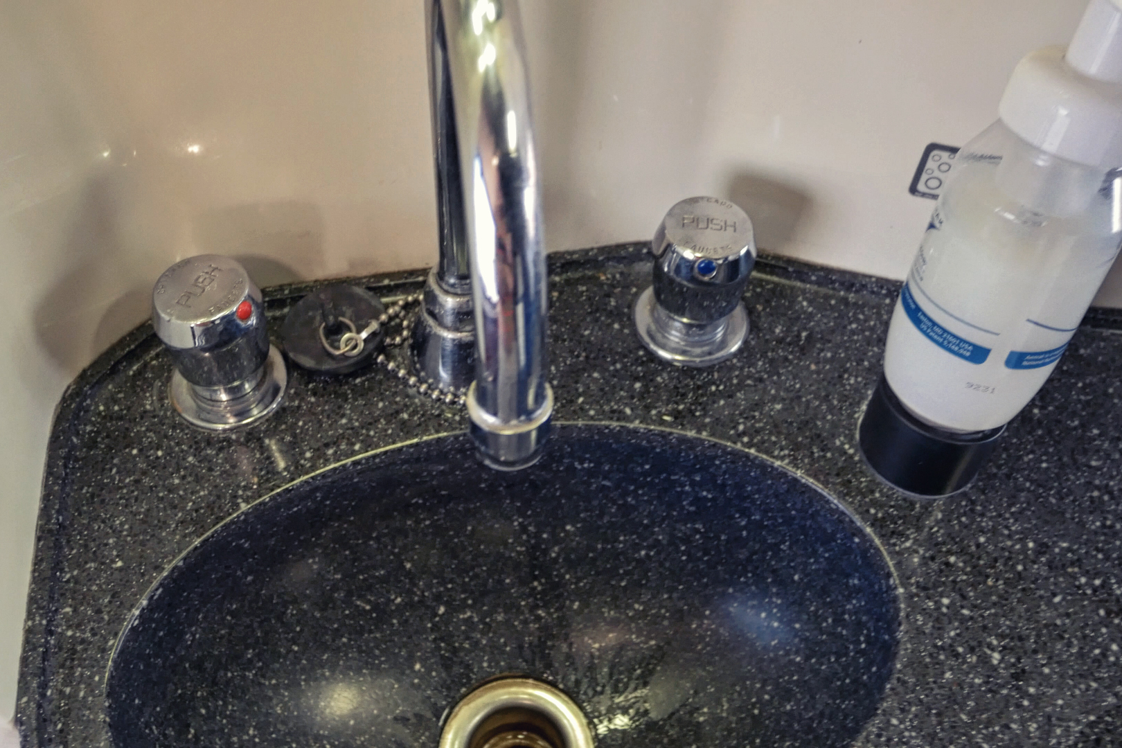
浴室可以免费使用,不限时间。内部如下,准备了毛巾,香皂。个人觉得空间对于火车来说已经很大了。使用体验:水量充足,温度可调,不过放换下来的衣服的空间似乎有点小。总的来说三天两夜的长途旅行,能在火车上洗个澡可以说是非常舒服了。
下层的家庭套间恰好空着,笔者就去拍了张照。家庭套房包括两张横向床一张纵向床,空间较大。
 家庭套房内部
无障碍房间可以给残疾人和陪护人居住,由于门关着,笔者无法进入。从结构图上看,里面应该含有一个无障碍卫生间。
至此,双层卧铺车Superliner的内部构造和细节就介绍完了,接下来,我们回归行程。
飞驰在平原
当地时间下午2点整,列车正点从芝加哥联合车站开出。随着芝加哥的高楼渐渐从视线中远去,出现在眼前的是广袤的平原。在第二天一早到达丹佛之前,列车会经过伊利诺伊州,爱荷华州,内布拉斯加州和科罗拉多州。这一段路的地形都比较平坦,使得我们可以欣赏到美国的平原风光。下面开始放图。
 芝加哥西部某地
 出了芝加哥就能看到平原的景色
 夕阳下残留着积雪的平原
夕阳西下,天上出现了美丽的晚霞。
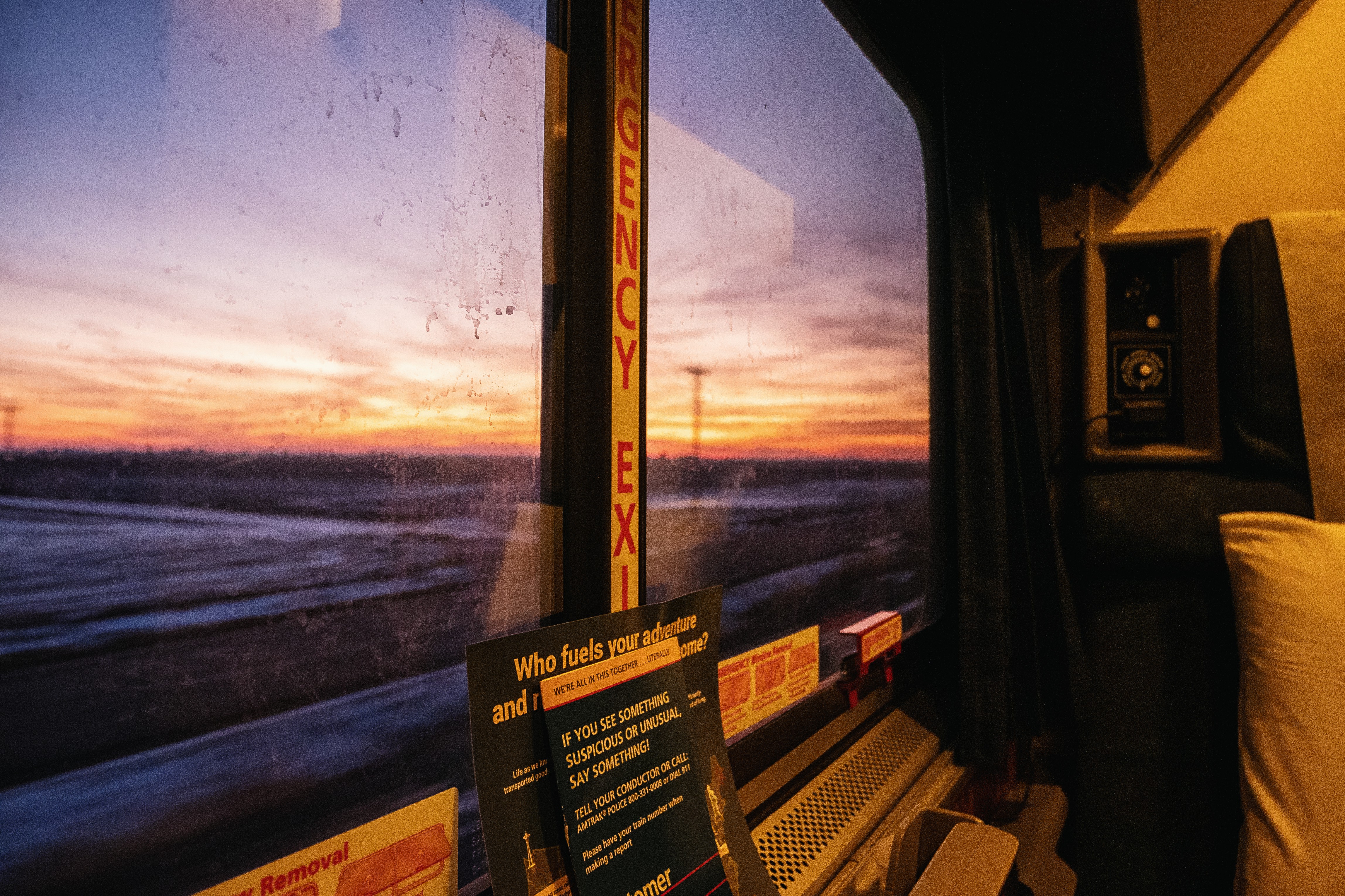 晚霞
晚霞
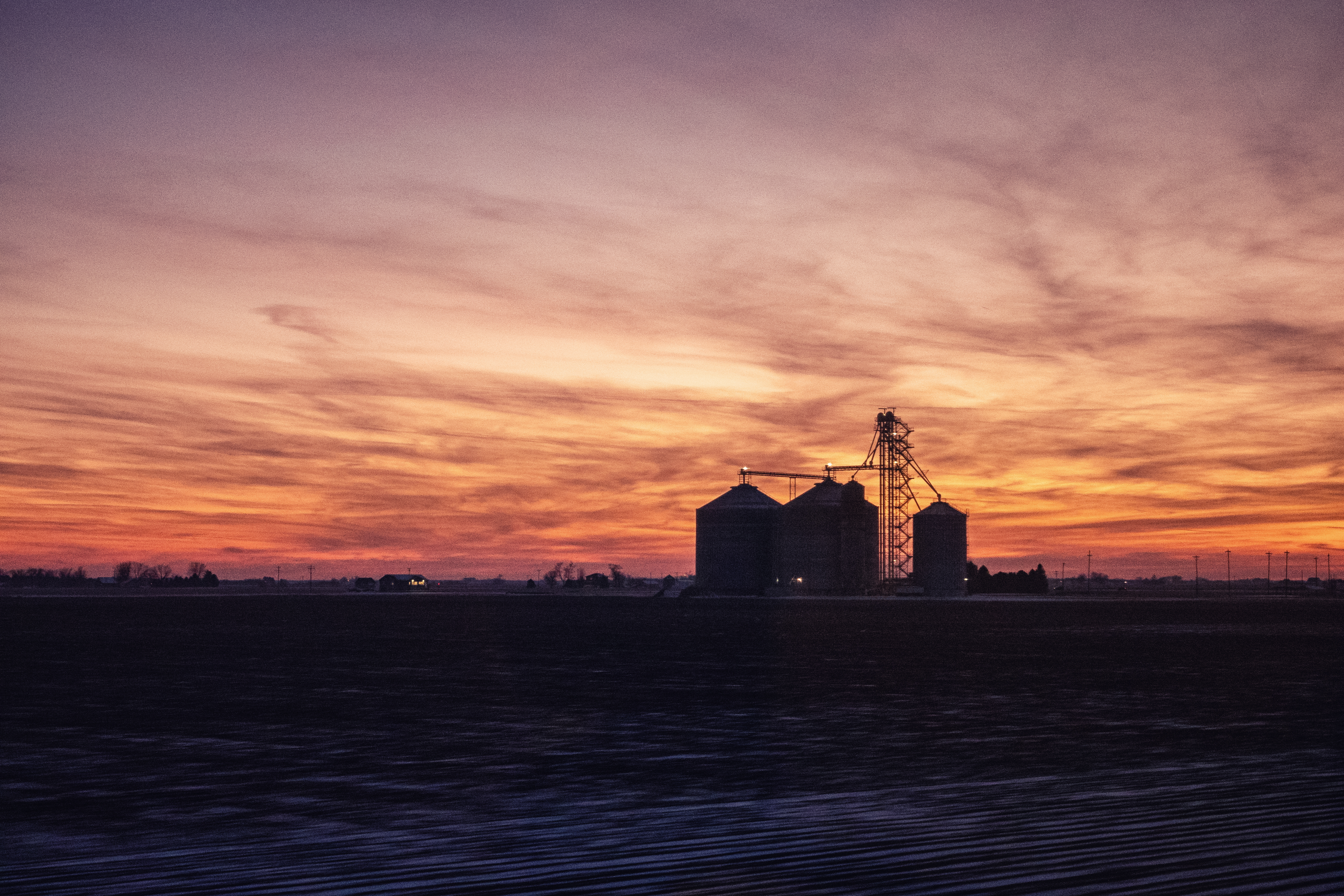 霞光笼罩下的景色
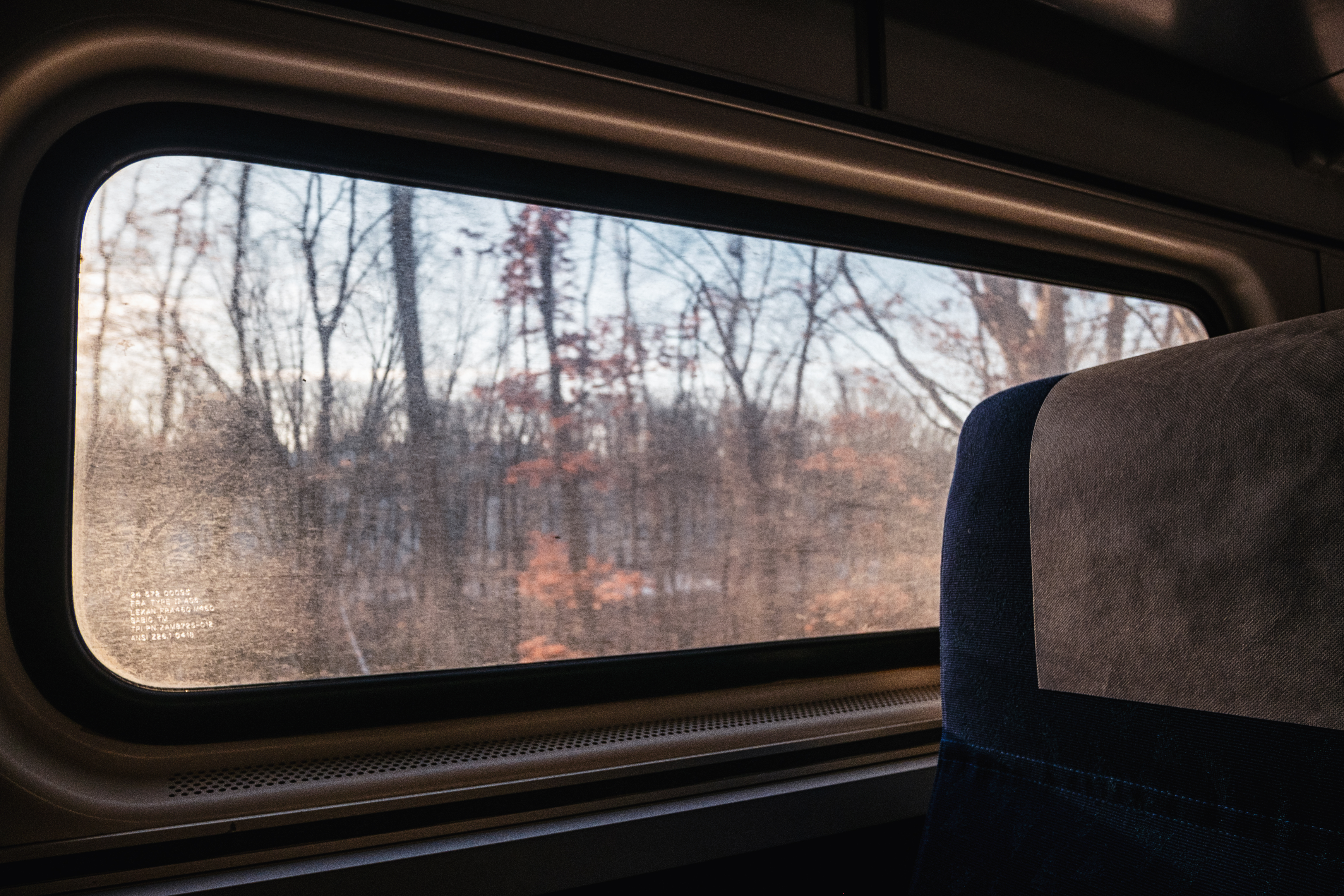
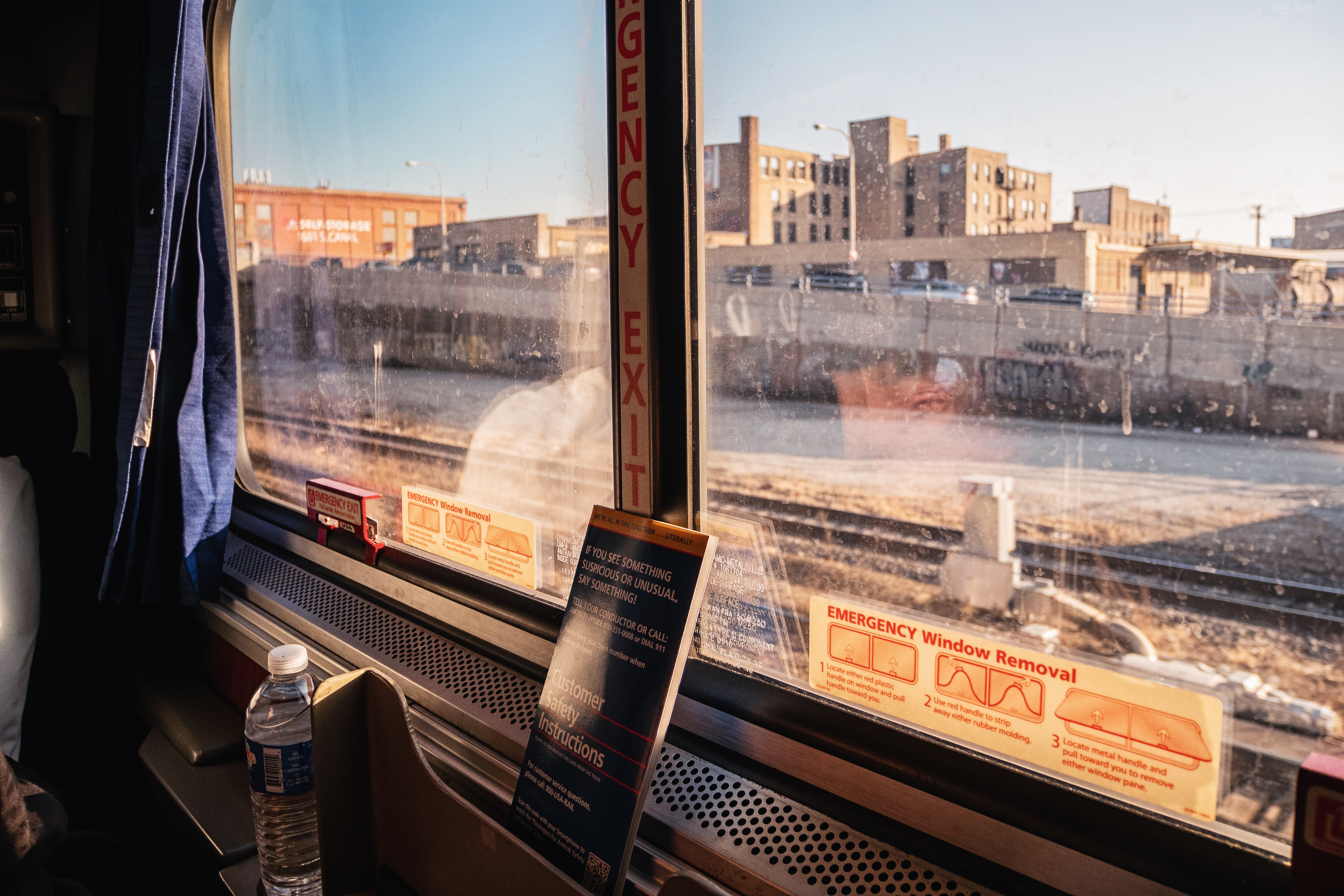
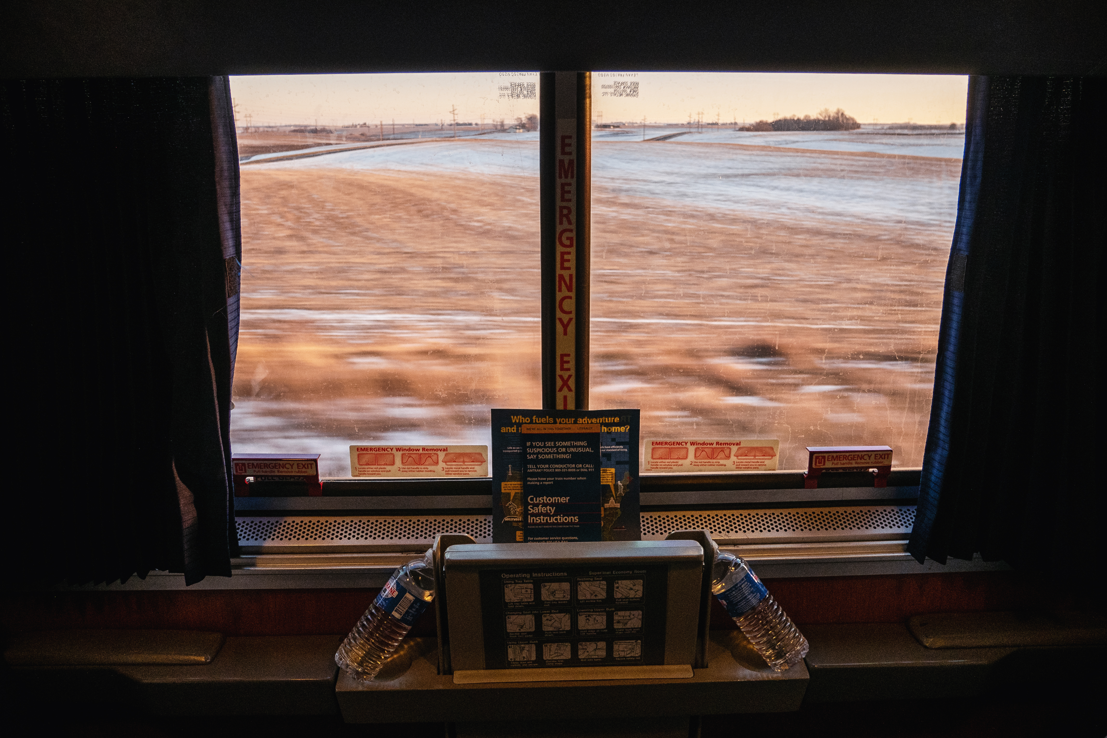
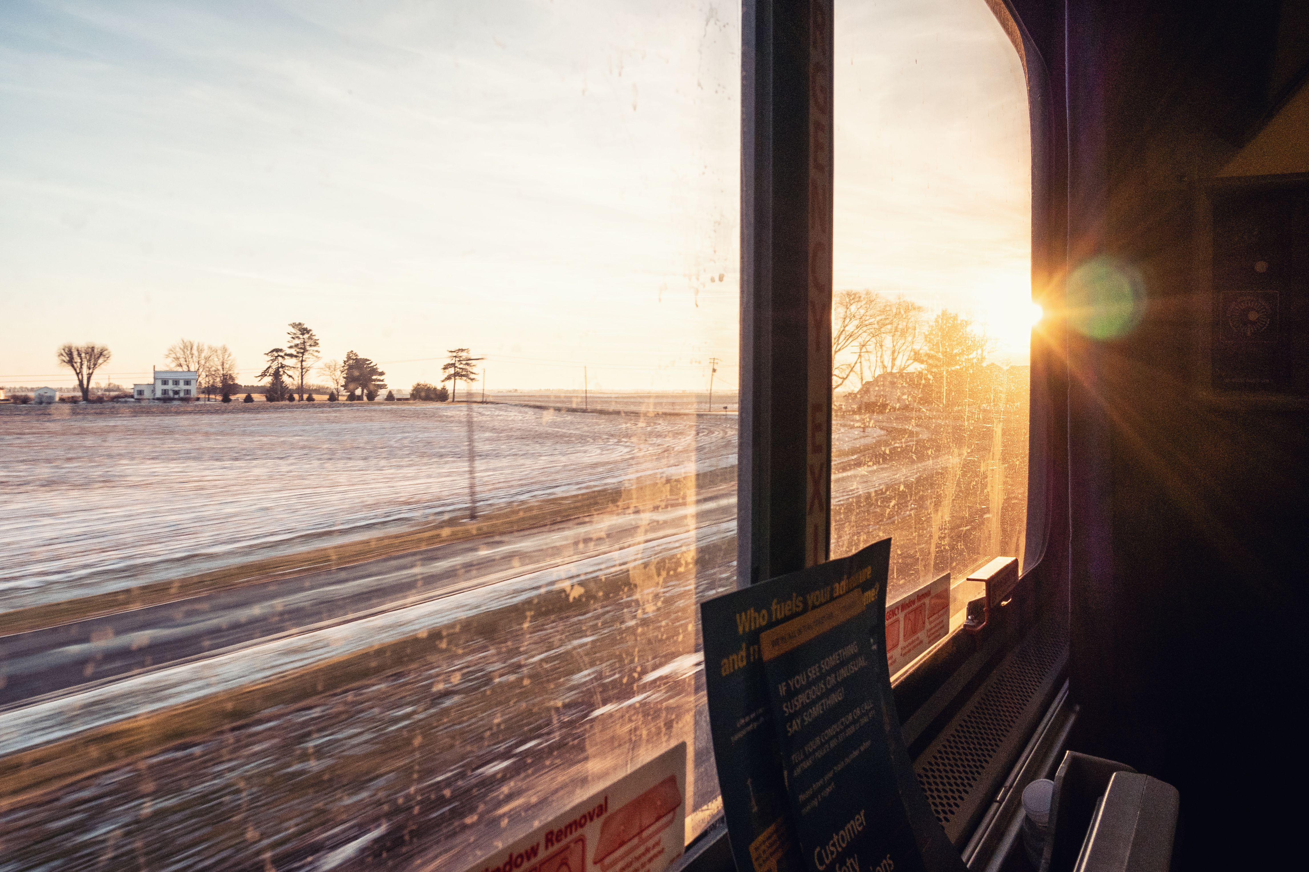
 车窗外流逝的风景
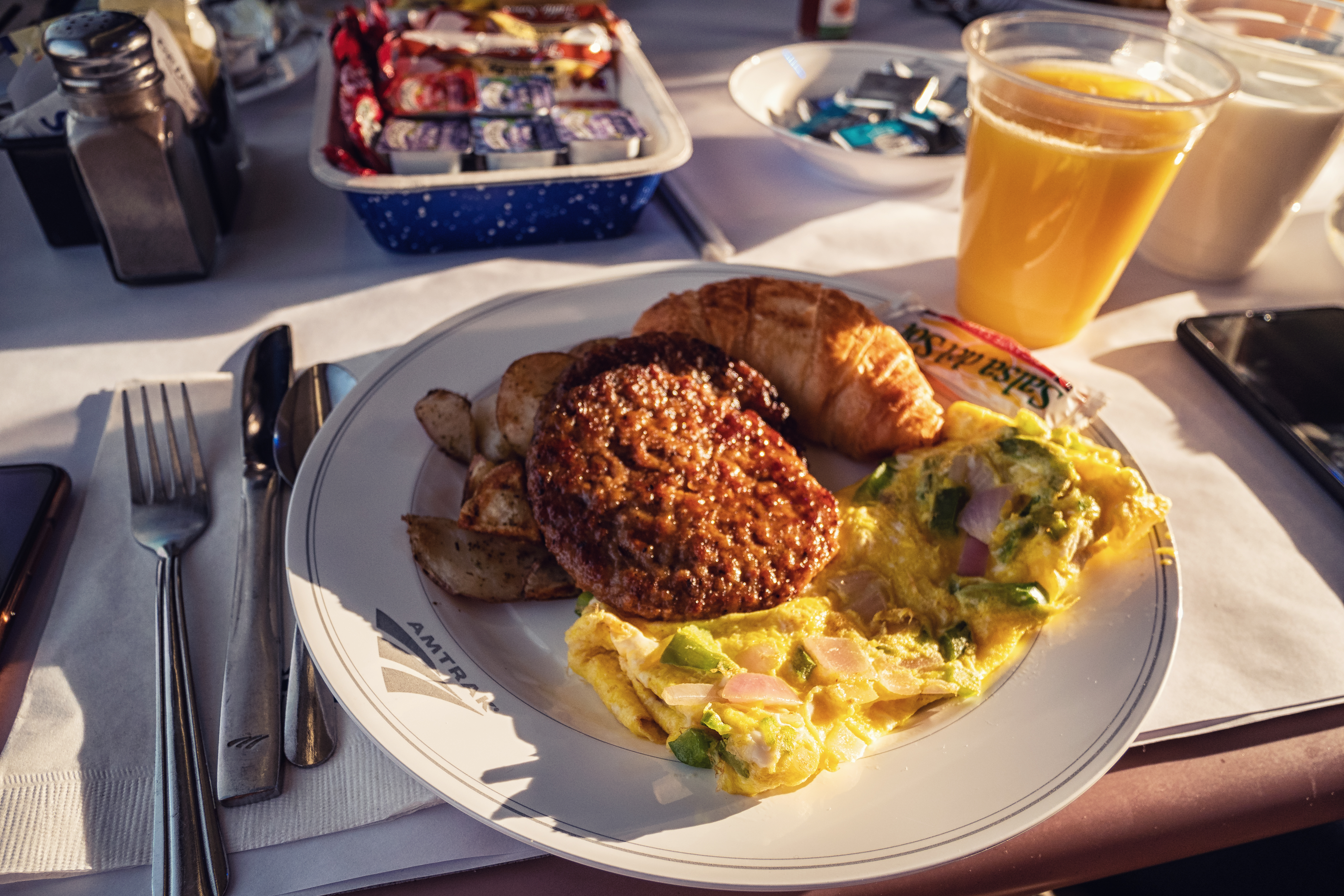
傍晚六点左右,我们前往餐车用餐。晚餐的时间是发车不久之后和自己车厢的列车员预约好的。放一下菜单,感觉还是非常丰盛的。早中晚餐都在同一份菜单上。菜单是手持着拿手机拍摄的,后期经过了透视矫正,部分区域比较模糊,还请见谅。需要高清版的话可以去文章末尾的链接区找美铁官方版菜单的链接。
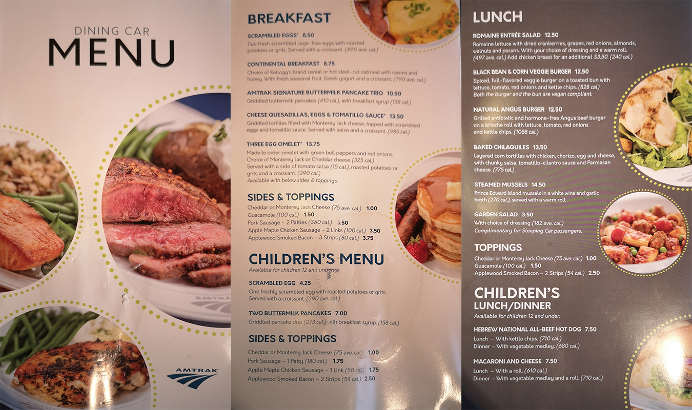 菜单1
菜单1
 菜单2
菜单2
费用看上去比较贵,不过持卧铺车票的乘客,除了酒和小费以外都是免费的。
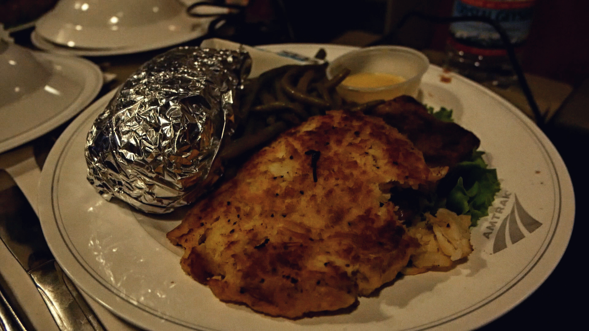
经过一番思考,笔者点了牛排(THE AMTRAK SIGNATURE STEAK),味道还是非常不错的。
 牛排,注意那个烤土豆很大,可以根据食量换成其他配菜
值得一提的是列车餐车采用拼桌的方式,由列车员安排和陌生人拼桌吃饭,一张餐桌四个人。在等待上菜和用餐的过程中就可以和同餐桌的人一同交谈。个人觉得这样的安排还是非常不错的,能够遇到很多不同的人,听到不同的事情。在几天的行程里,我们就遇到了去中国旅行过的夫妇,在和我们同样的城市(安娜堡)工作的情侣,第二次乘坐加州和风号只为在不同季节看落基山风景的夫妇等等。我们交换了美食情报,讨论了旅行见闻,他们还给出了很多我们之后行程的建议。其中的一对老夫妇,我们在旧金山游玩之时再度偶然碰面,可以说是很巧了。
 餐车内的样子,基本每桌都是四人,本图是在我们对面的人入座前拍摄的
饭后,我们回到房间,打算早点休息,毕竟第二天列车会翻越落基山脉。翻越落基山脉的行程可以说是全程中风景最好的一段,我们要保存充足的精力来观景。
夜渐渐深,列车行驶在广袤的平原上。伴着列车的哐当声,怀着对明天的期待,我们进入了梦乡。
 展开后的下铺
翻越落基山脉
第二天早上七点不到,我们被闹钟叫醒。注意列车是向西行驶的,由于时区的变更,每晚都会往回调一小时,所以可以有一小时的额外睡眠时间(如果乘坐向东行驶的列车就要合理安排睡觉时间了)。醒来时,列车已经接近丹佛了,日出的天空被染成紫色,很是好看。
 平原的日出
平原的日出
早上七点五十分左右,列车到达了丹佛车站,比预计的时间晚点了四十分钟左右。前一天刚刚经历了两个小时的晚点,四十分钟实在算不上什么。值得一提的是,丹佛车站是尽头站,因此列车需要经过一番操作,然后倒车进入车站。
 倒车进入丹佛车站的列车
列车在丹佛车站的停车时间较长,于是我们决定去站台上透个气。这次只是匆匆路过,下次如果还有机会的话,笔者还是希望好好到丹佛来玩一玩的。
 停靠在丹佛车站的列车
 向车头方向看去
 站台上也可以看到丹佛的通勤铁路列车
回到列车上,我们先去餐车吃了个早饭。美式的早餐比较简单,但味道还算不错。在用餐的过程中,列车从丹佛车站驶出,向落基山脉进发。
 早餐
早餐
吃完早餐,我们赶紧前往观景车厢。此时的观景车已经有很多人。观景车有两种类型的座位,一种是和餐车一样的四人的桌子,另一种是纵向的直接面对车窗的座位。我们到的时候,只剩下为数不多的四人桌的座位。
 我们的座位,请忽略同学的相机和电脑,以及实在有点脏的窗玻璃
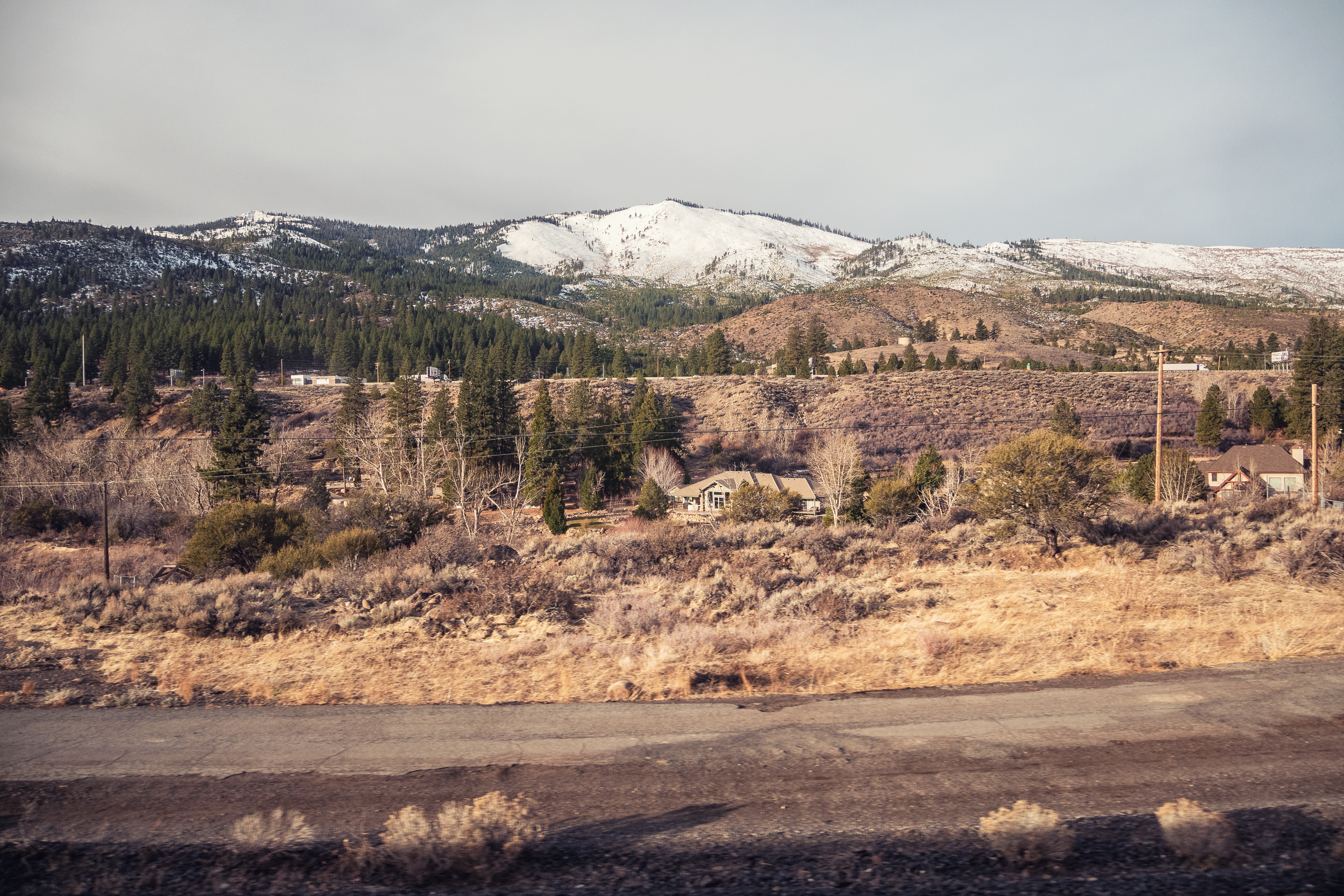
列车从丹佛车站开出后不久,地形不再是之间的平坦,开始出现了起伏。
 丹佛郊外某地
 列车通过弯道,可以清楚的看到车头,请忽略后期都救不了的反光
爬坡的过程中风景非常不错,乘客们纷纷掏出自己的设备拍照。随着海拔逐渐升高,线路边的积雪也逐渐变得多了起来。
 回望远处的丹佛市区
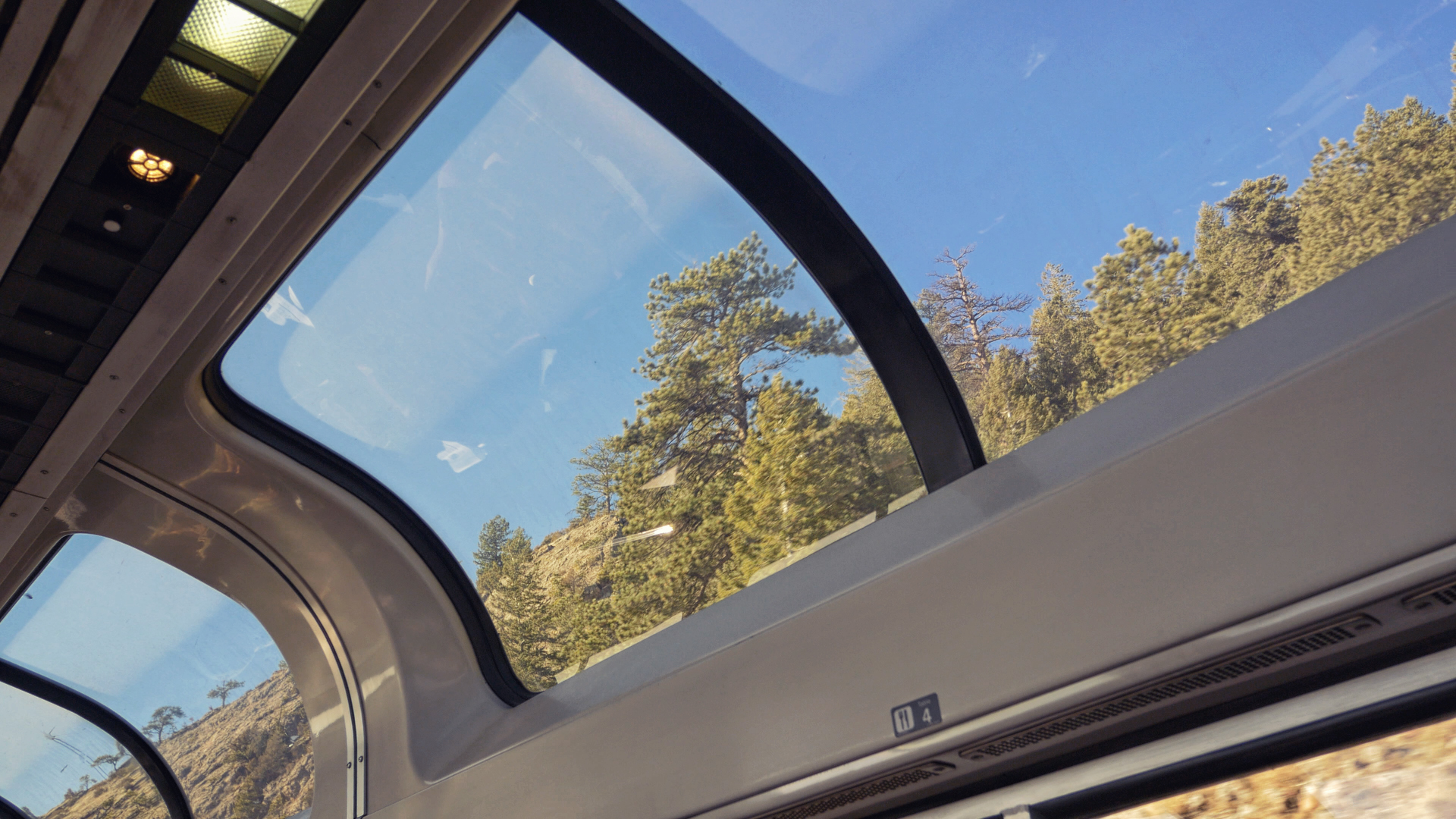 上层车窗提供了更广阔的观景空间
 半山腰的风景
 讨论着风景的乘客
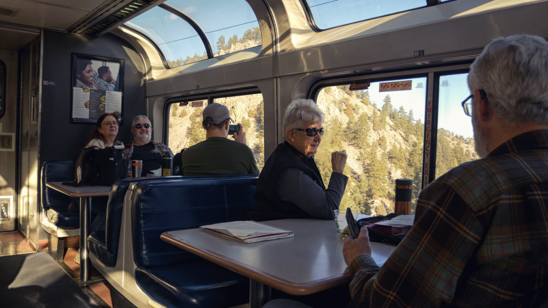 欣赏风景的乘客
 爬坡中的列车
 越来越多的积雪
随着深入山区,线路经过的隧道也不断增多。其中比较有名的一个是Moffat隧道,这个十千米长的隧道极大的减少翻越Rollins pass的路程(由于没有找到中文译名,所以保留了英文)[4]。列车在途经这些观景点的时候,都会有相应的解说。
从Moffat隧道穿出之后,车窗外已经俨然一片雪国的景象。列车在积雪覆盖的山间穿行。看着这样的景色,暂时放下一切尘世的繁琐(不是矫情,只是手机没信号(/ω\)),总觉得能让身心得到极大的放松。不由自主的拍了一大波图,下面开始图片轰炸。
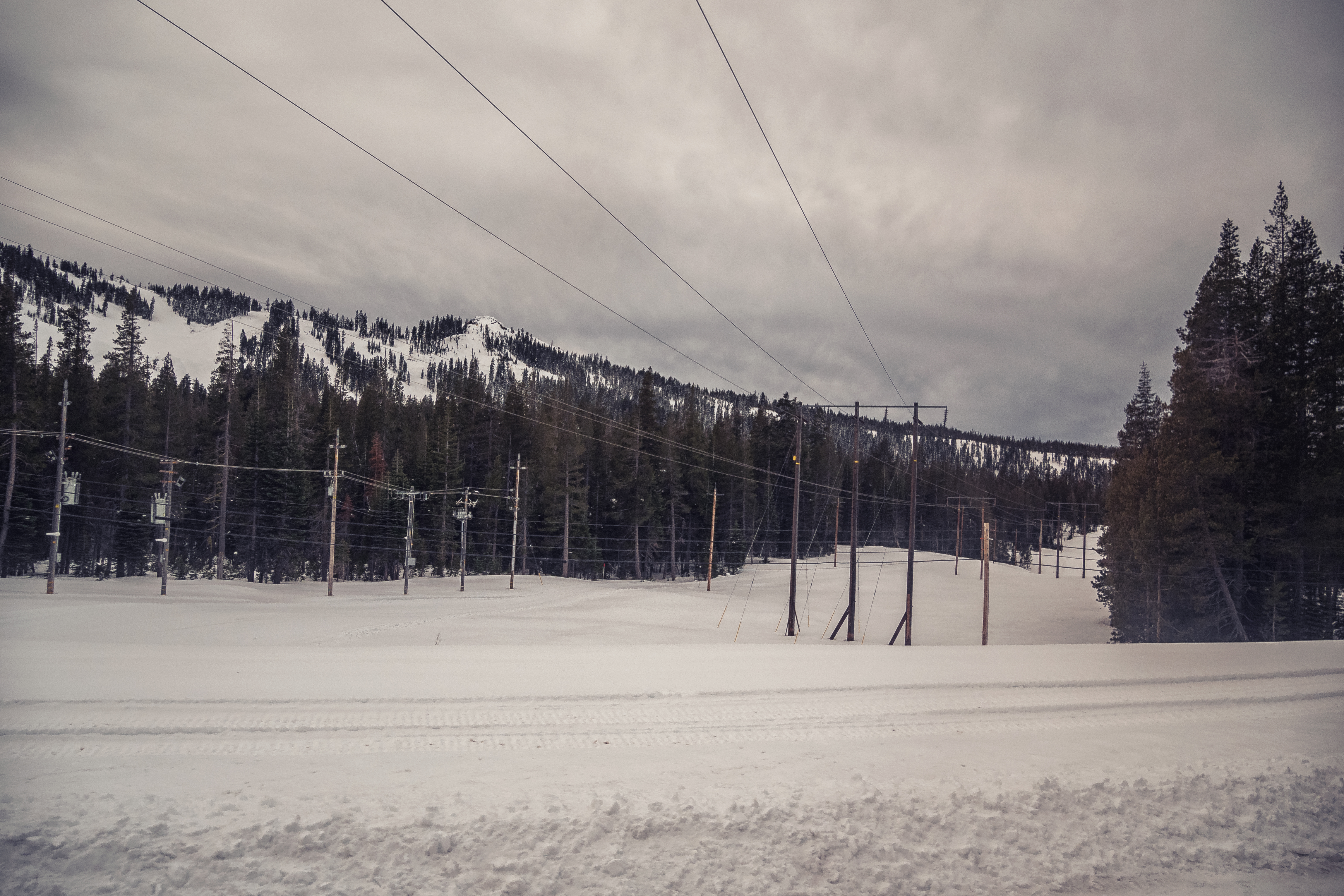
 从Moffat隧道钻出就能看到Winter Park Resort滑雪场
 观景车的上层车窗可以提供更广视野,用来看天空和山上的岩石非常不错
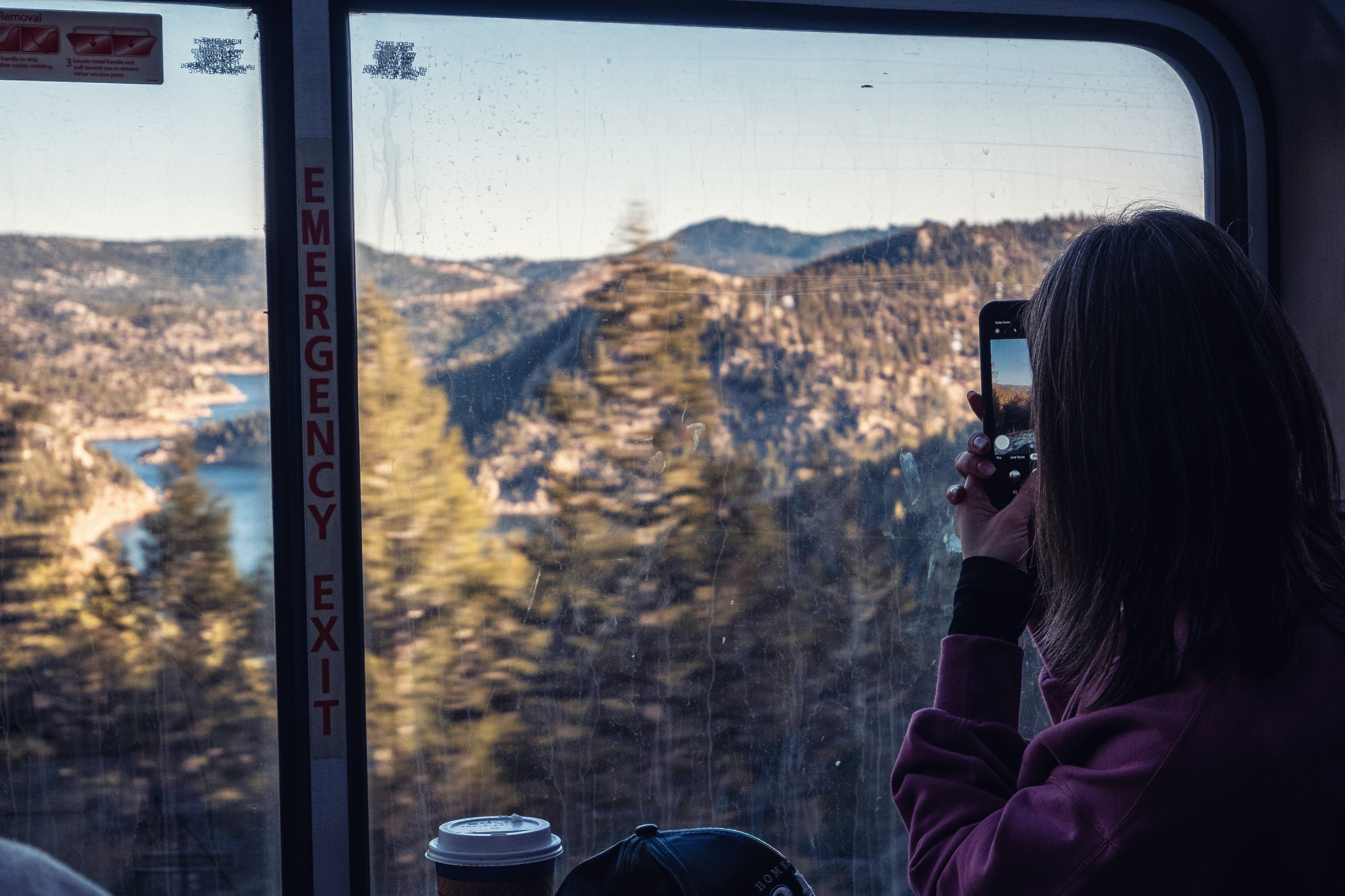
 观景车内观景的乘客
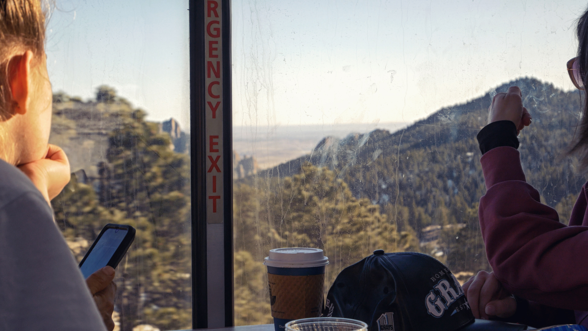
 观景车内观景的乘客,这一部分就是之前说的直接面对车窗的座位
 面对车窗观景的乘客们
 车窗外的风景
 远处的雪山,可惜玻璃反光严重
 远处的雪山
远处的雪山
 停靠某车站时拍到的景象
 和汽车竞速,由于小半径曲线多,速度时常是赶不上汽车的
 在河谷中蜿蜒的线路
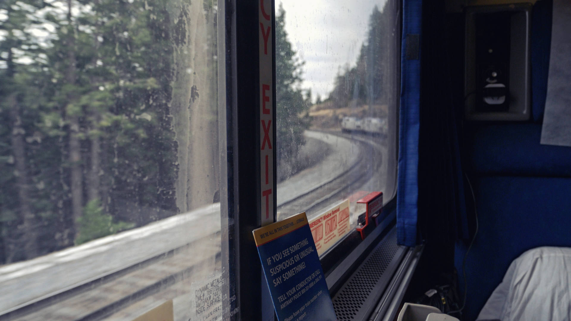
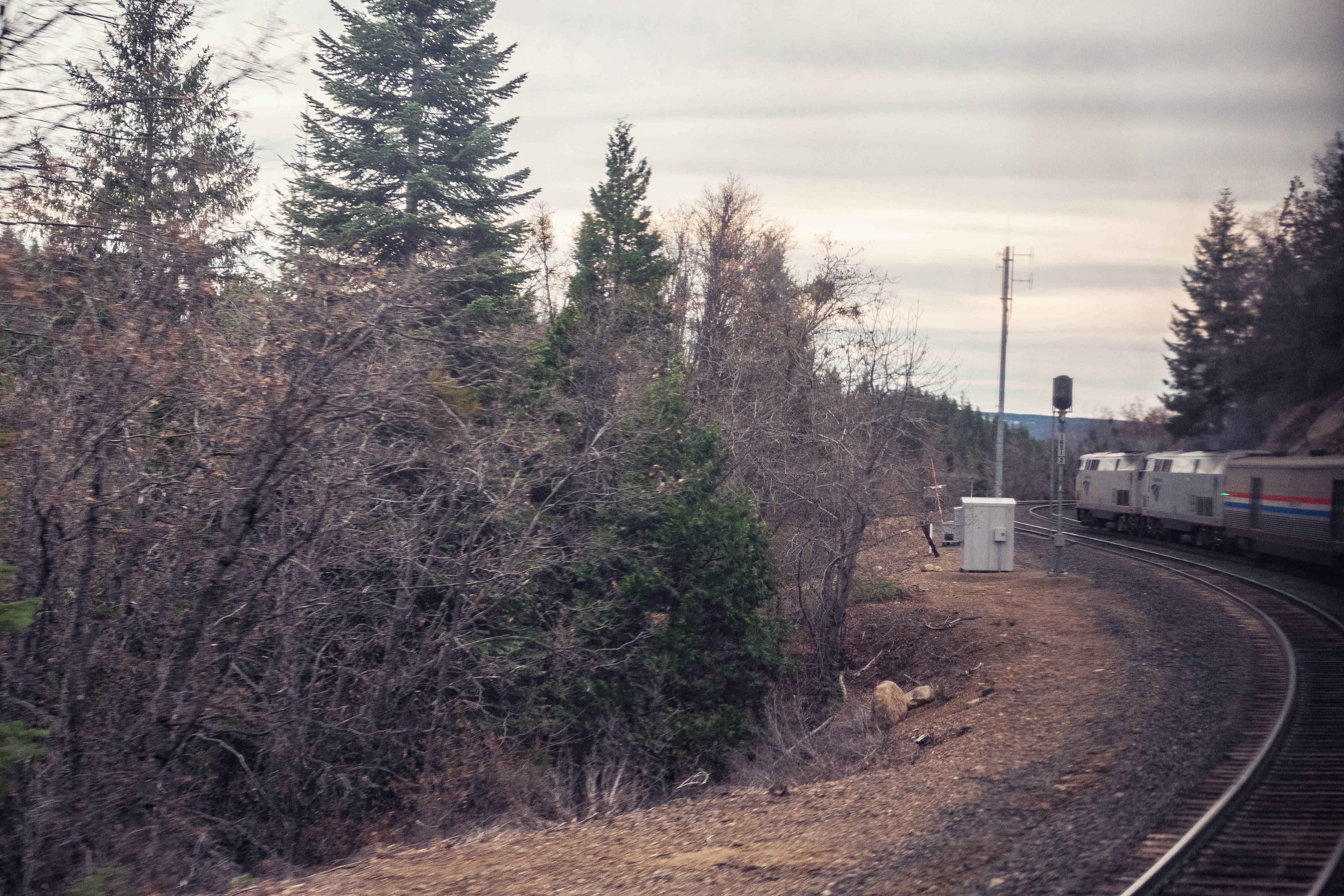
 小半径曲线多,时常可以看到车头两台可爱的P42DC
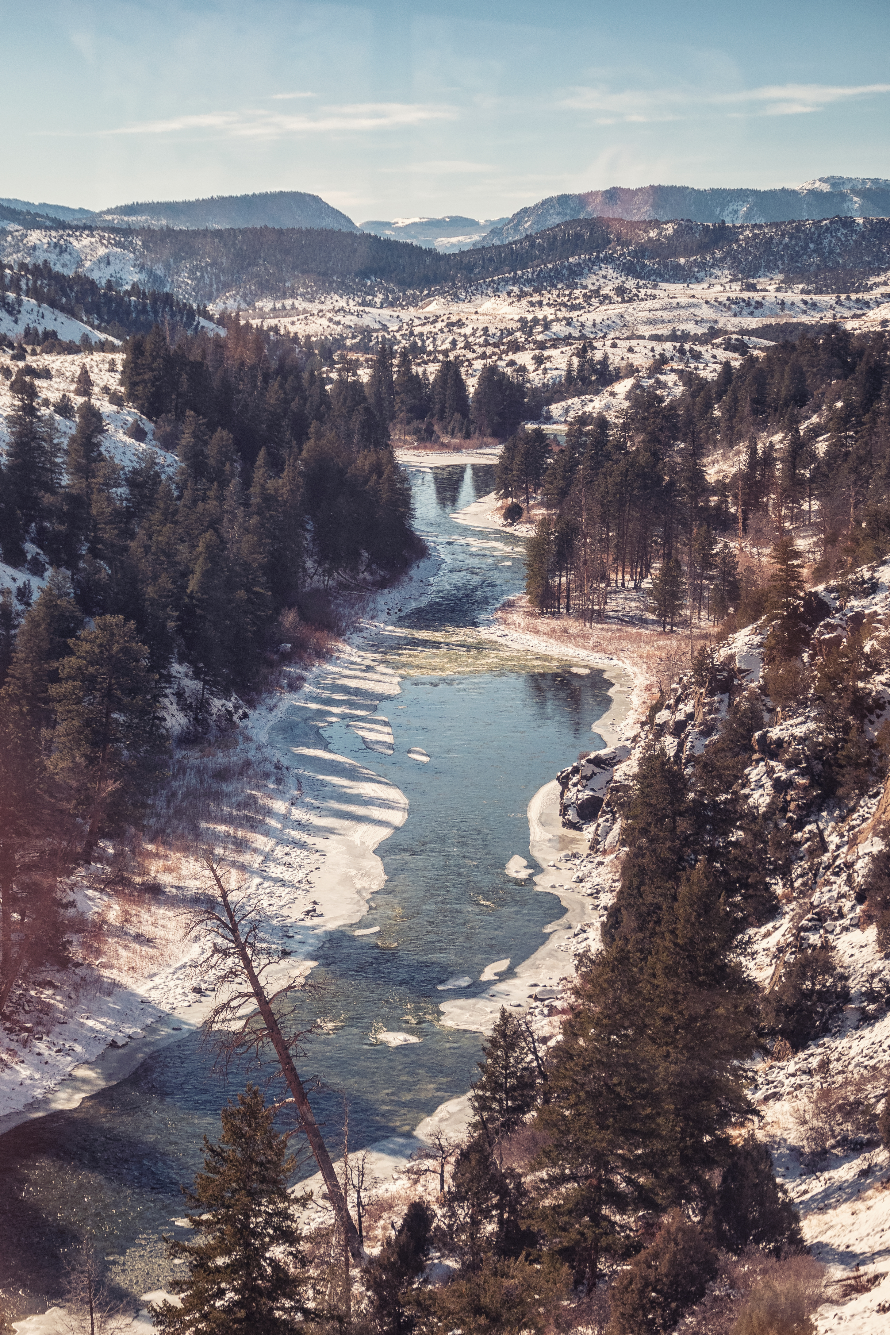 科罗拉多河,很长一段路列车都是沿着河谷穿行的
 雪山下的河流
 穿行在山间的列车
 和同学拍了整个上午
从早上到中午,我们一直待在观景车内。沉浸在美丽的风景中,不觉时间过的很快。中途去观景车楼下的小卖部买了点零食饮料,所以午饭就拖的比较晚。下午两点左右,我们前往餐车去吃午饭。和晚饭略有不同,午饭不是找自己车厢的列车员预约的。餐车的列车员会在广播通知可以开始午饭预约,然后乘客前往餐车预约,列车员会按照预约的先后顺序广播叫人去餐车用餐。
因为实在是不想吃汉堡和沙拉,笔者就点了一个Chilaquiles,查了下应该是墨西哥风味的料理。这个料理并不难吃,但不是非常合笔者的口味。
 Chilaquiles
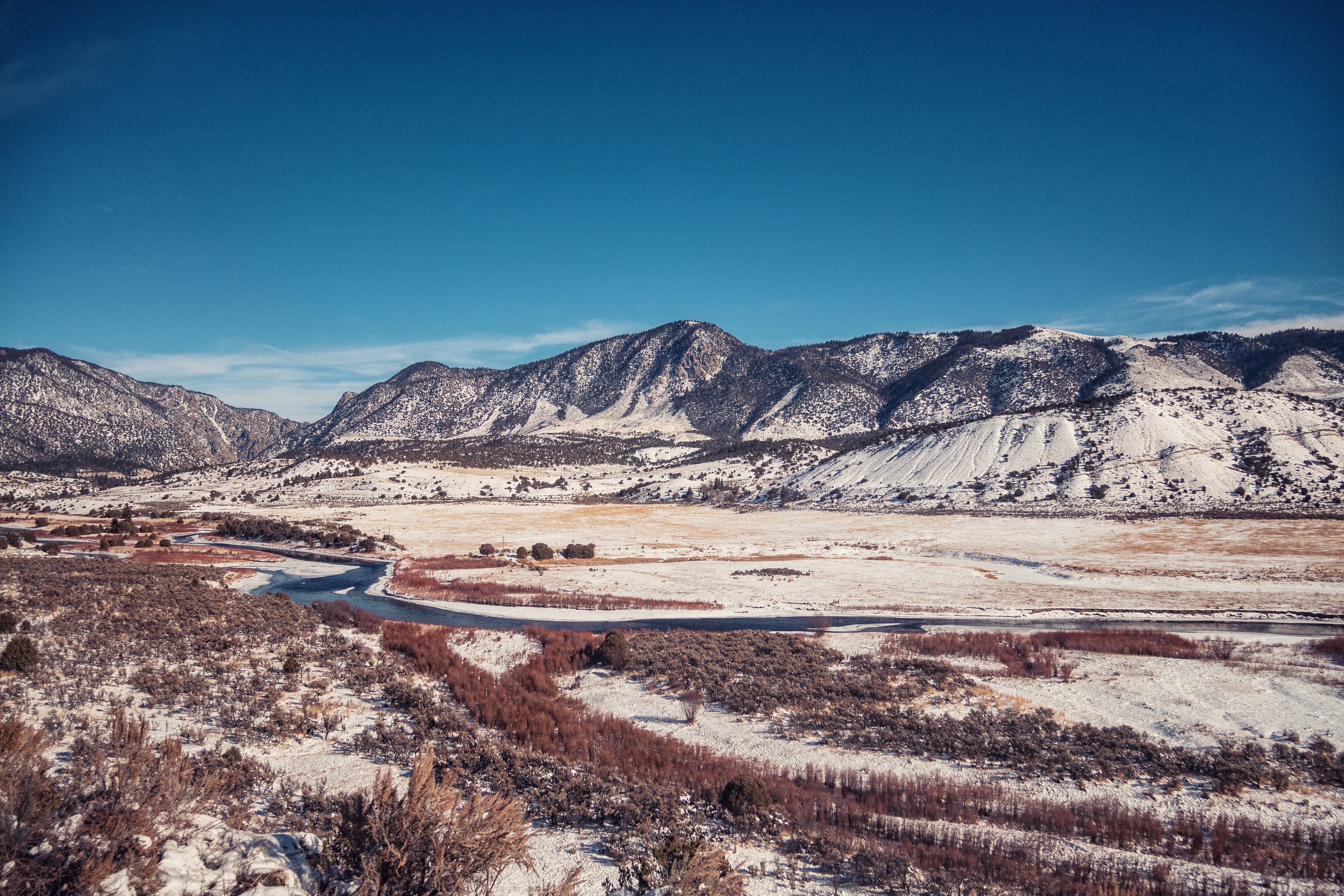
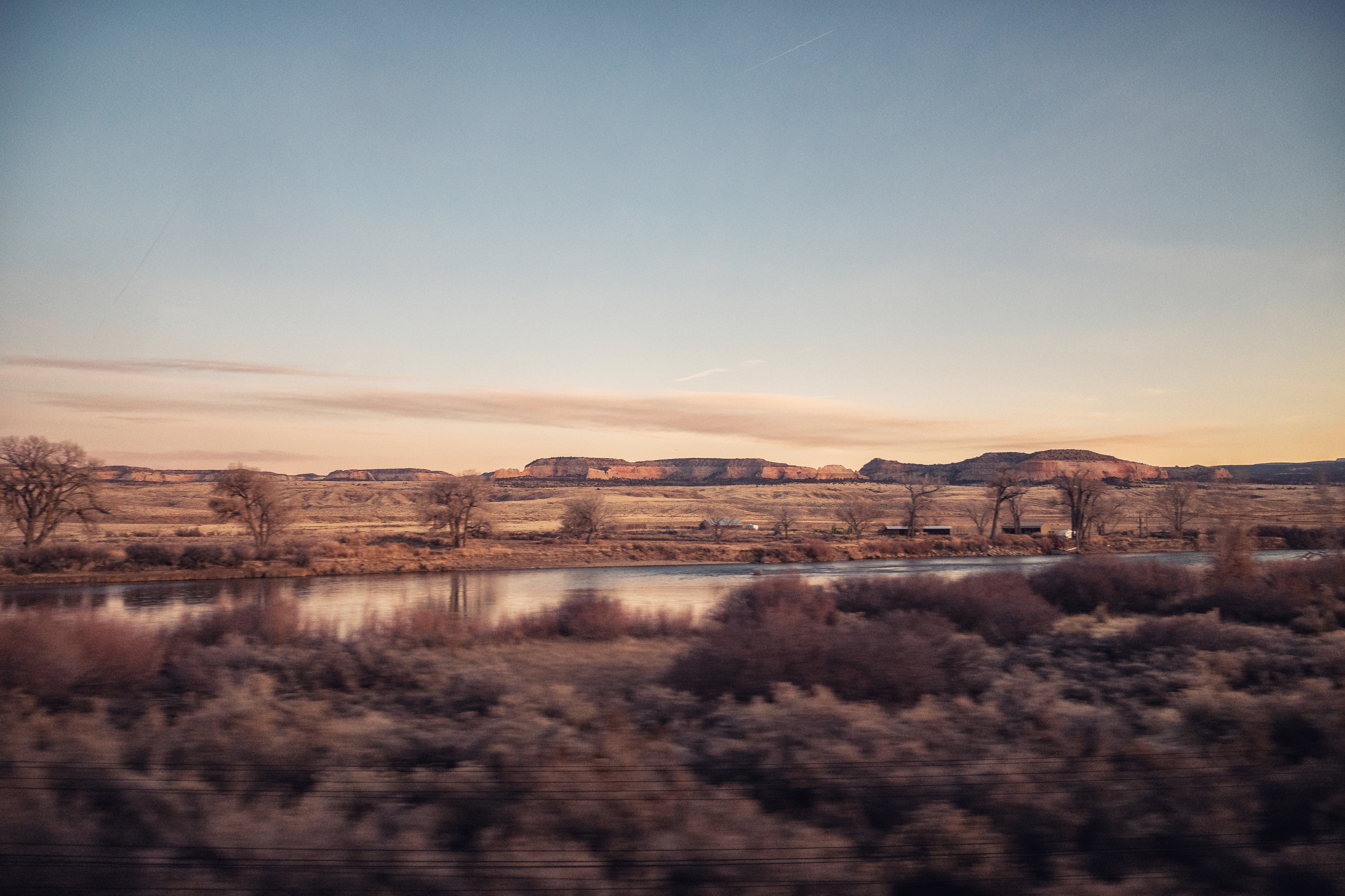
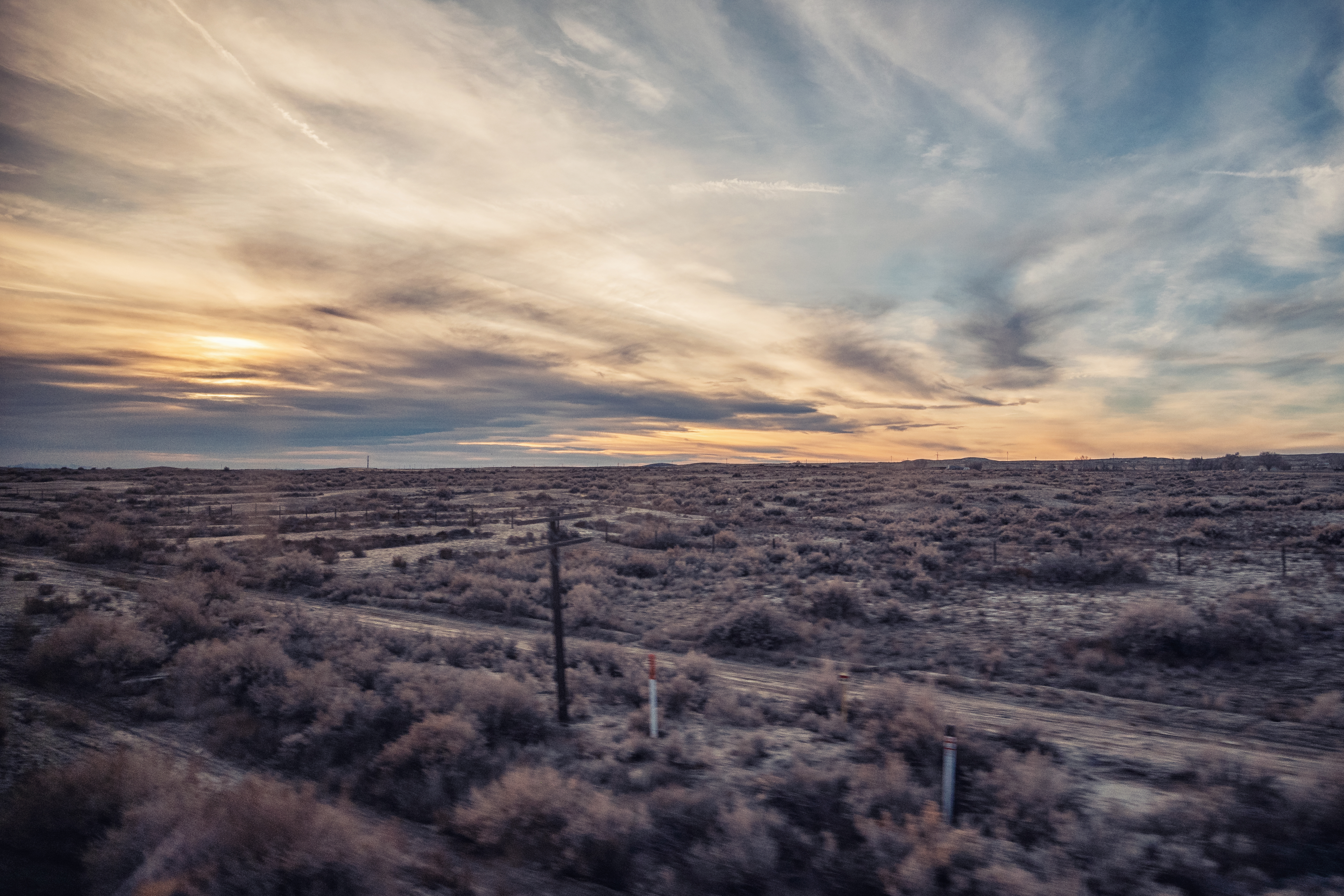
饭后,我们回到了自己的房间继续看风景。此时,列车逐渐离开洛基山脉,窗外的积雪逐渐减少,地貌也又一次发生了改变。以红色的土地为标志的沙漠地貌出现在了视线中,说明我们来到了科罗拉多高原。
 科罗拉多河
科罗拉多河
 红色的土地
红色的土地
 科罗拉多河
科罗拉多河
 列车逐渐离开山脉
 地貌逐渐发生变化
傍晚时分,列车从科罗拉多州进入犹他州,夕阳照在沙漠的砂岩孤峰上,呈现出好看的橙红色。
 橙红色的窗外
 橙红色的窗外
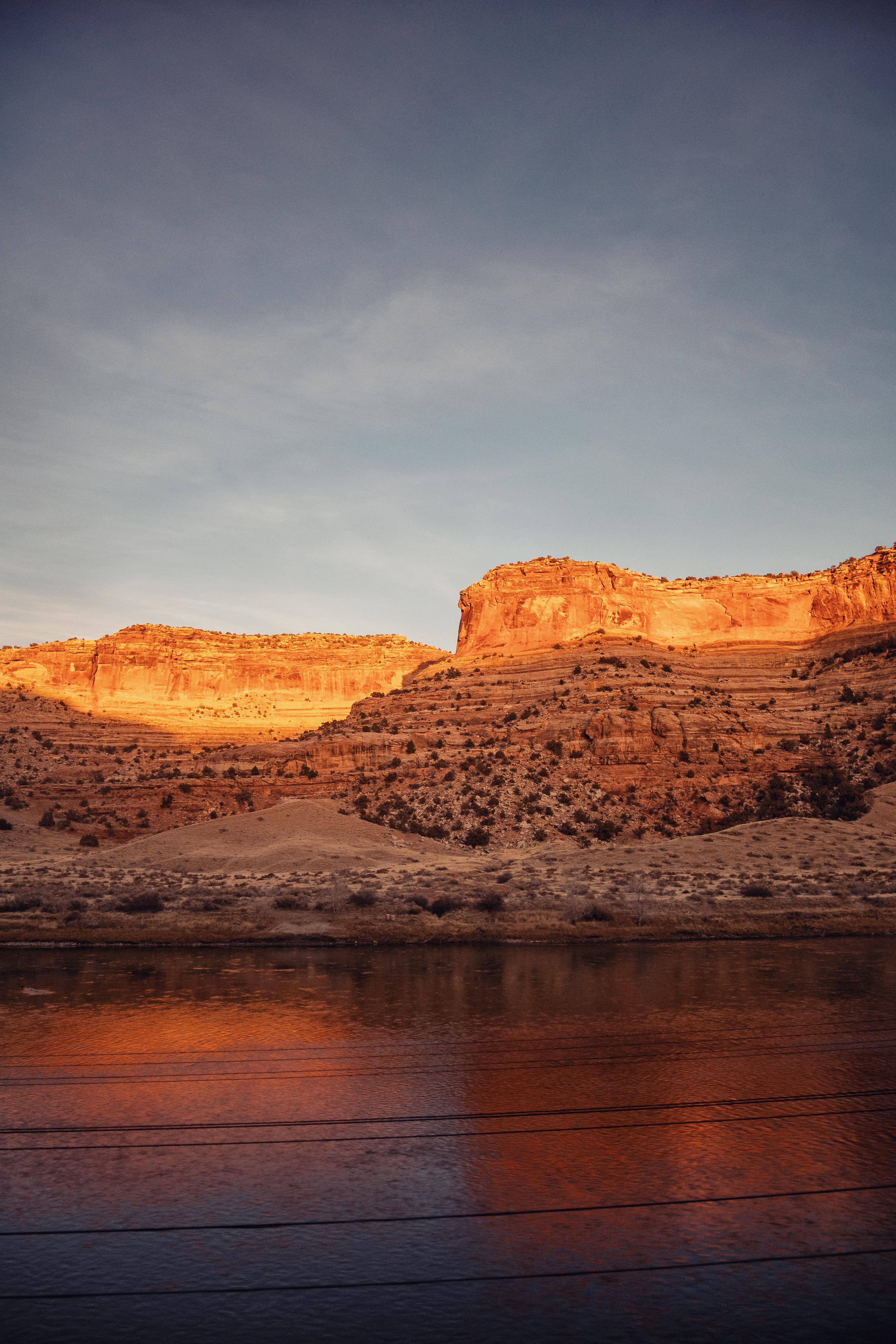 好看的橙红色
 远处的孤峰很是好看
夕阳西下,又到了用餐的时间。这一次晚餐,我们没有去餐车用餐,而是选择了让列车员把我们点好的餐点送至房间来。这一次,笔者点了Land & Sea Combo,翻译成中文的话大概是海陆套餐。如此高端的名字背后,也只是比昨天的牛排多了个蟹饼而已。不过既然不要钱,多吃一些也挺好。味道的话,一如既往的不错。
 沙漠上的夕阳西下
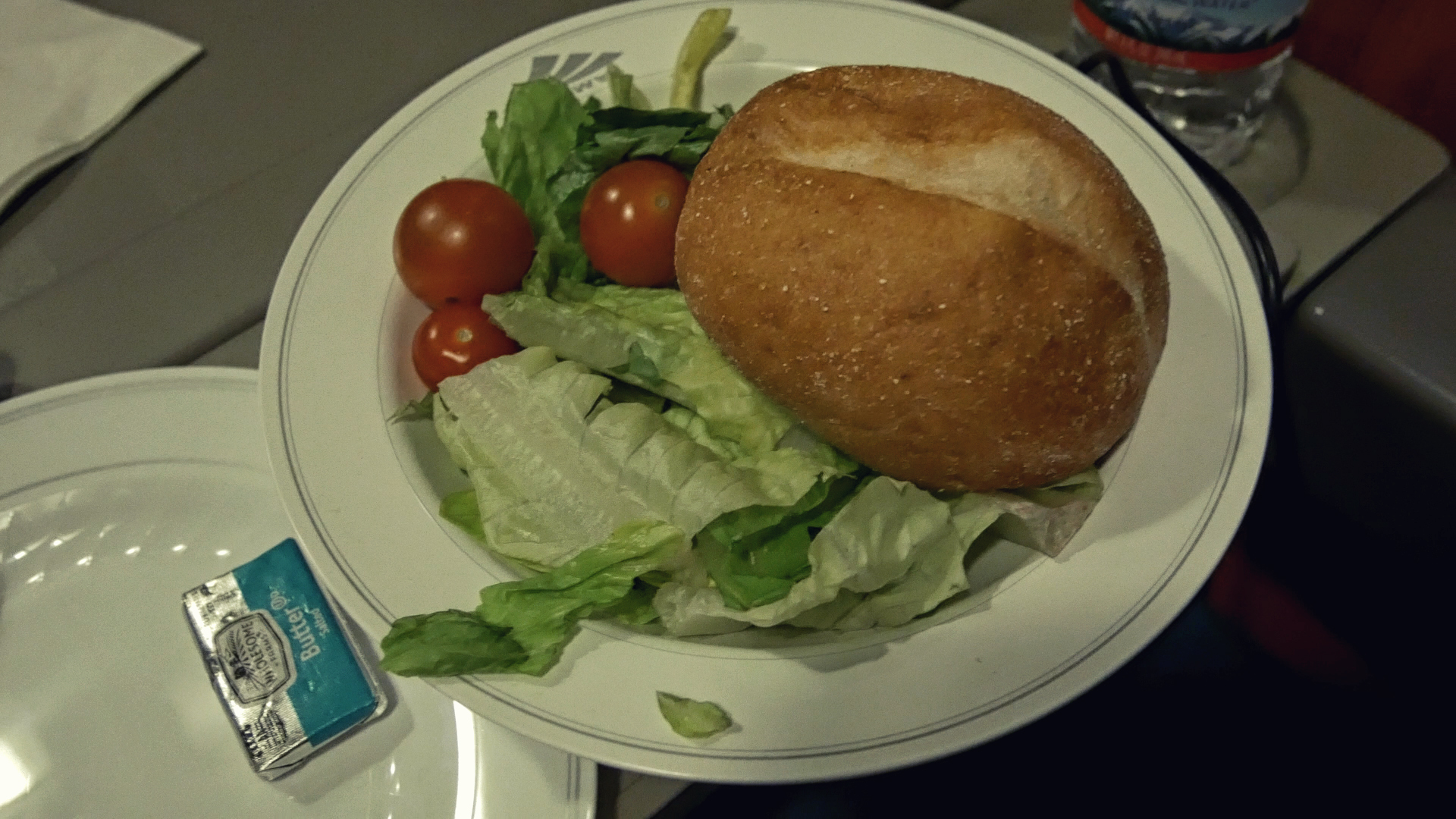 作为配菜的沙拉和面包
 正餐,视频截图,画质差,还请见谅
晚上十一点左右,列车还算正点的到达盐湖城。顺便一提,到达盐湖城之前的一段路风光也是非常不错的,不过我们的列车是在夜色中经过。乘坐东行列车的话可以看到这一段的风景。这一段经过士兵山峰(Soldier Summit)的线路比较有名,被收录在了TS游戏里(游戏里有加州和风号的任务,不过用的还是上一代列车的编组)。
经过了一天的观景,我们都比较疲惫,决定早点休息。在借着手机热点“决战盐湖城”之后,我们便去浴室洗了个澡,打算睡了。我们轮流睡上下铺,今天轮到笔者睡上铺。
 决战盐湖城
决战盐湖城
 上铺的样子
上铺的样子
睡在上铺,列车的抖动似乎比下铺更加剧烈一些,不过这样的抖动倒是很催人入睡,笔者很快就进入了梦乡。
到达加州
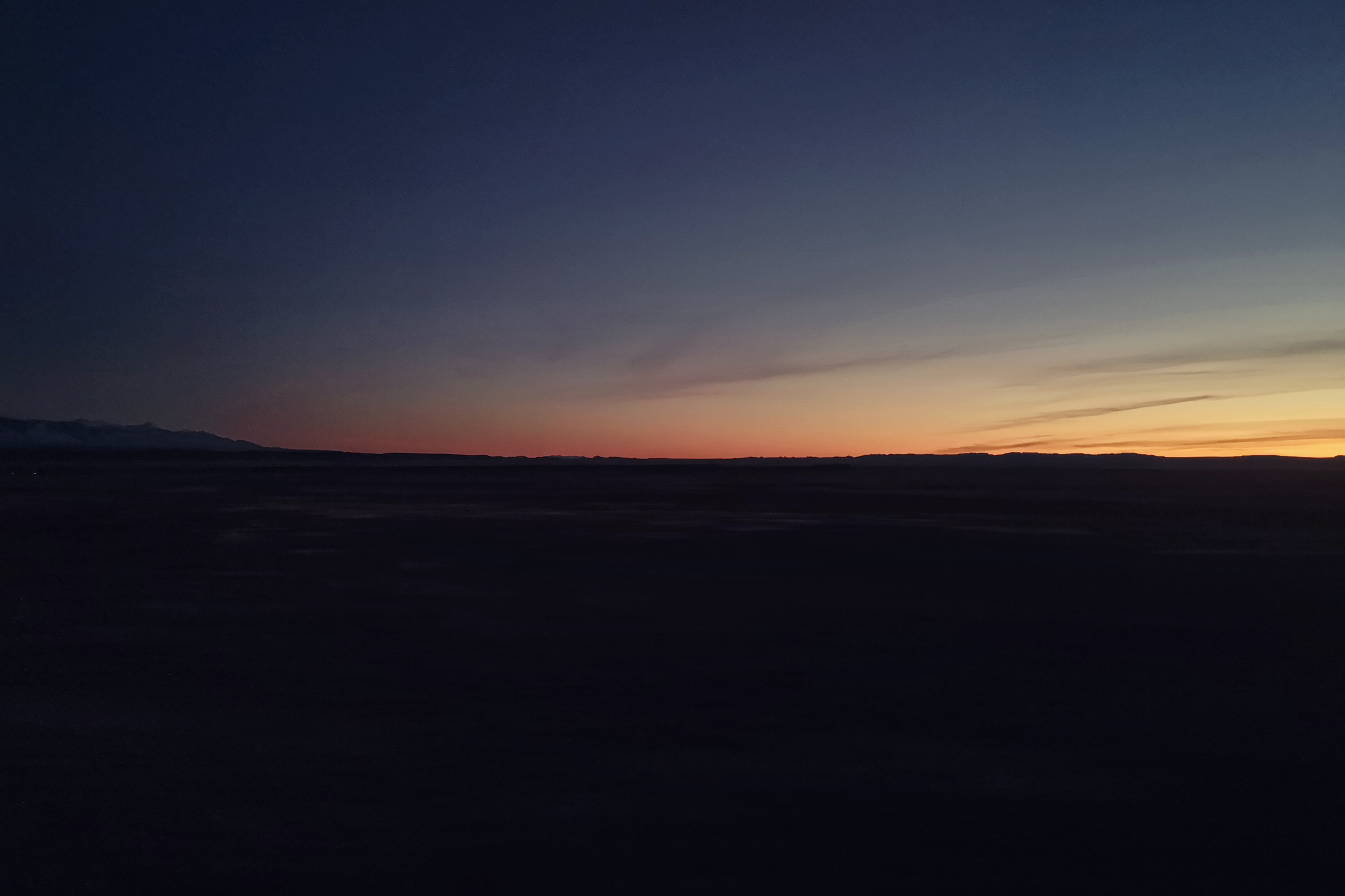
第三天早上,我们睡到自然醒。起床时,列车正接近内华达州和加州的交界处。
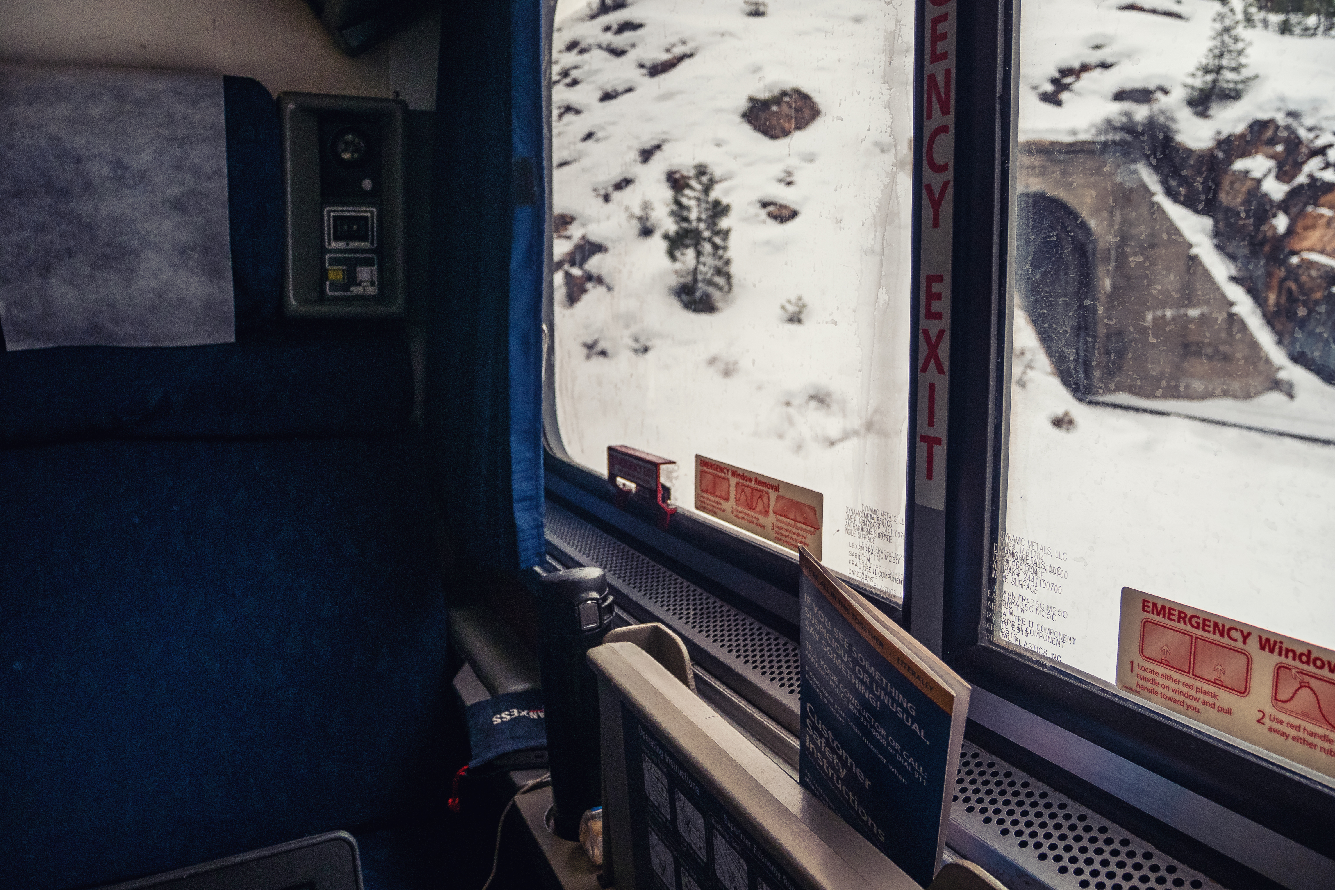
 车窗外的荒漠
去餐车吃个早饭。此时列车已经开始翻越加州东侧的内华达山脉。边吃早饭边看看风景,很是悠闲。
 依旧是很美式的早餐
 清晨的阳光洒在餐桌上
 一边用餐一边欣赏美景
回到自己的房间,列车已经穿行在了山间。可能是山间的天气比较阴沉,笔者还是更加喜欢前一日翻越落基山脉的风景。因此翻越内华达山脉的时候没有拍很多照片。
 白雪覆盖的窗外,附近也有滑雪场
 列车穿行在山间
 列车穿行在山间
 依旧是很多小半径的弯道
之后又去餐车吃了午饭。由于去的比较晚,到的时候有的菜品已经卖完了,于是点了一个蒸贝(Steamed Mussels)。味道比较普通,不过遇到了在同一桌吃饭的热情大叔和老爷爷,向列车员借来了一种酱,撒上之后味道变得好吃很多。
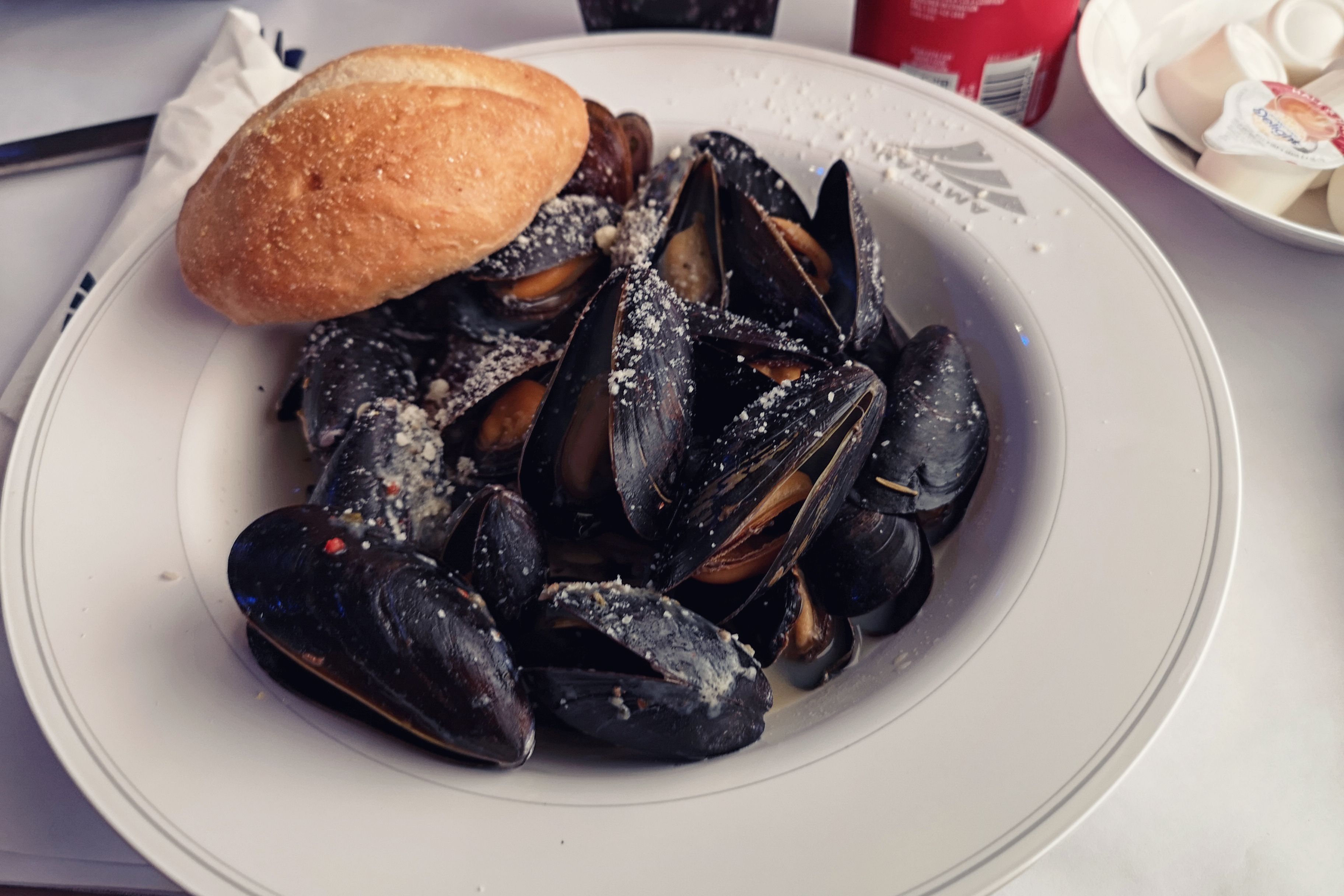 午餐
午餐
吃午饭的时候列车到达了萨克拉门托,意味着旅程只剩下两小时不到的时间。
 萨克拉门托
萨克拉门托
列车从萨克拉门托开出之后,我们也开始收拾随身物品,而列车继续向旧金山飞驰而去。
 车窗外的景象,天气比较阴沉
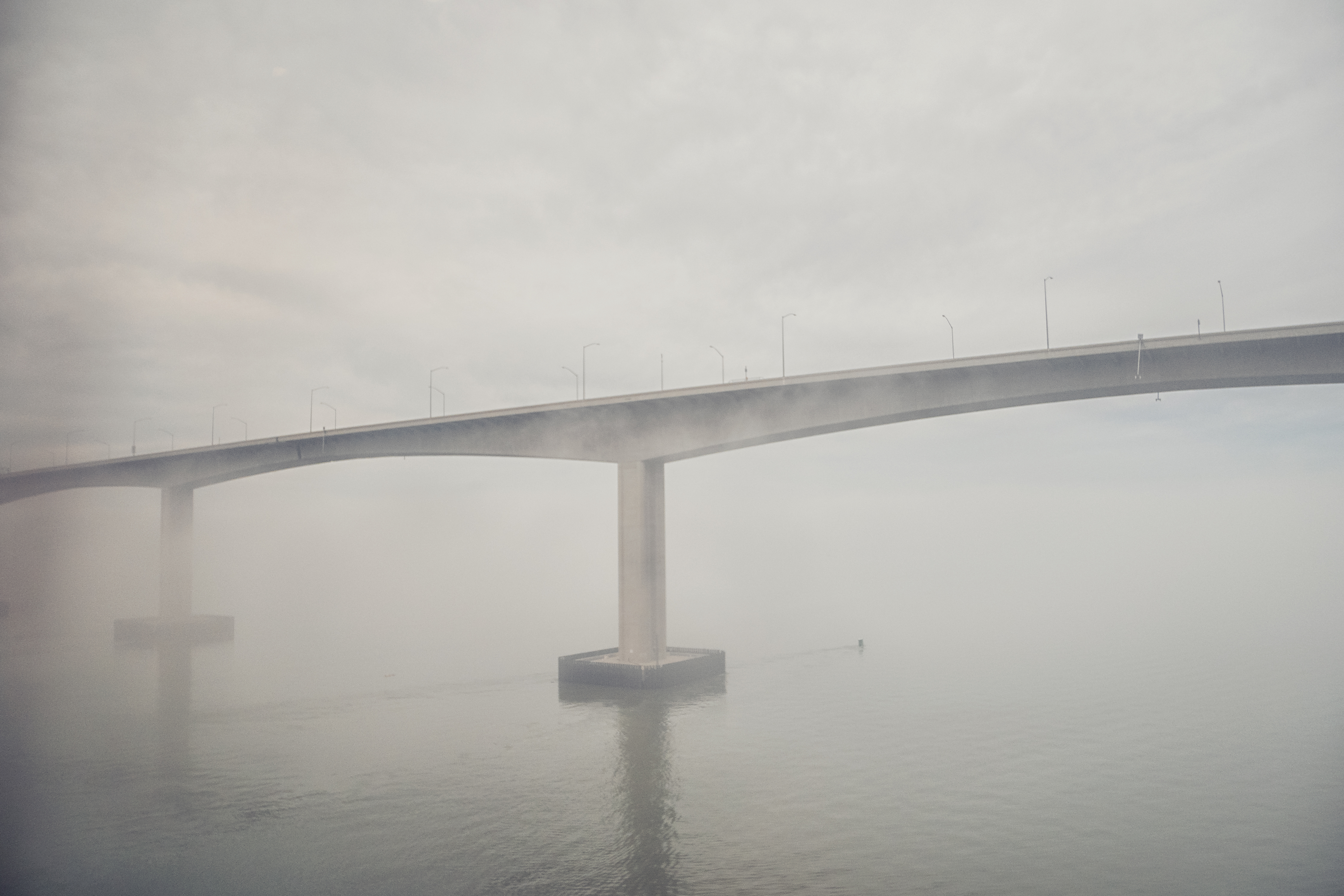 一座笼罩在雾气里的大桥
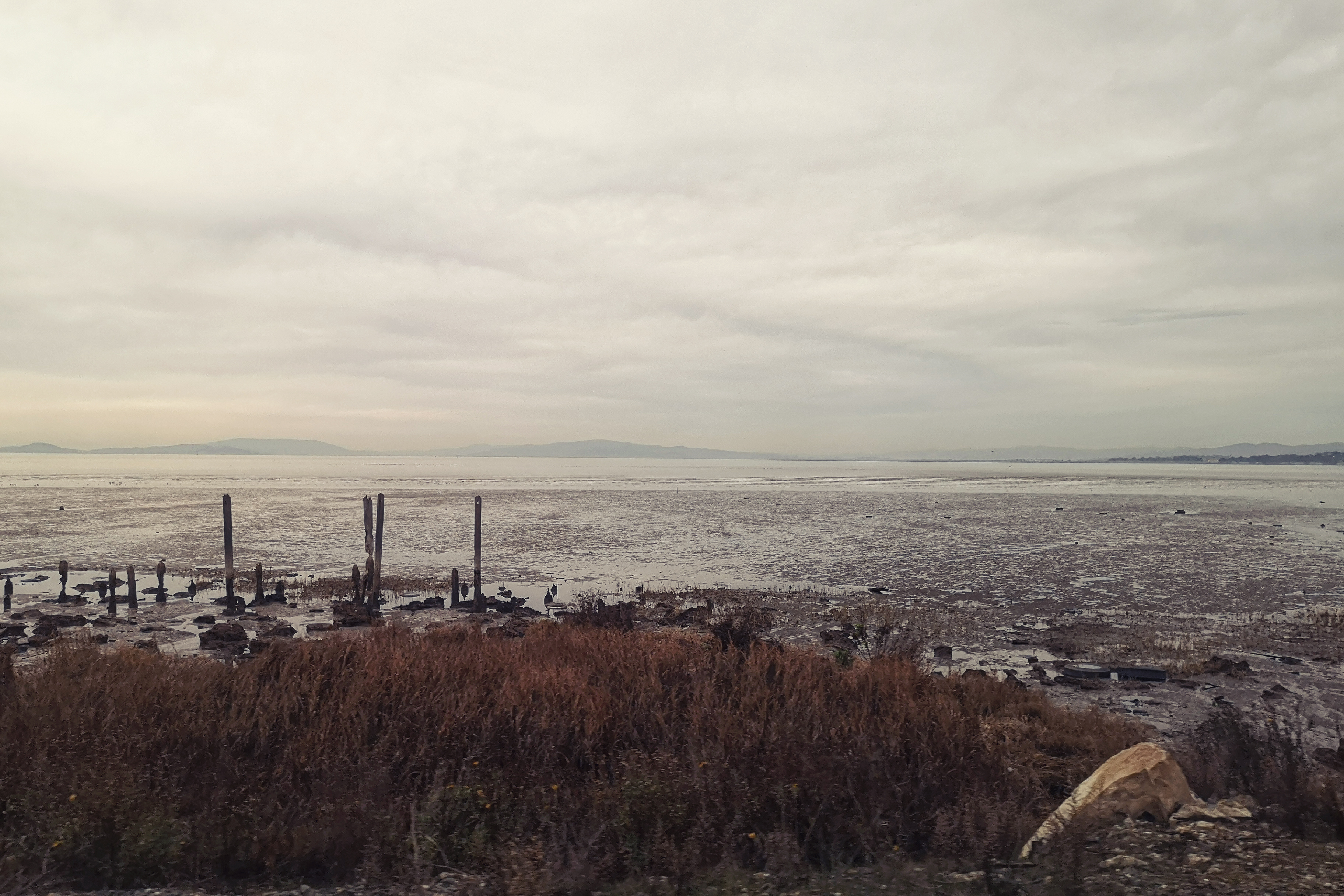 里奇蒙附近,列车沿着海湾运行,风景不错
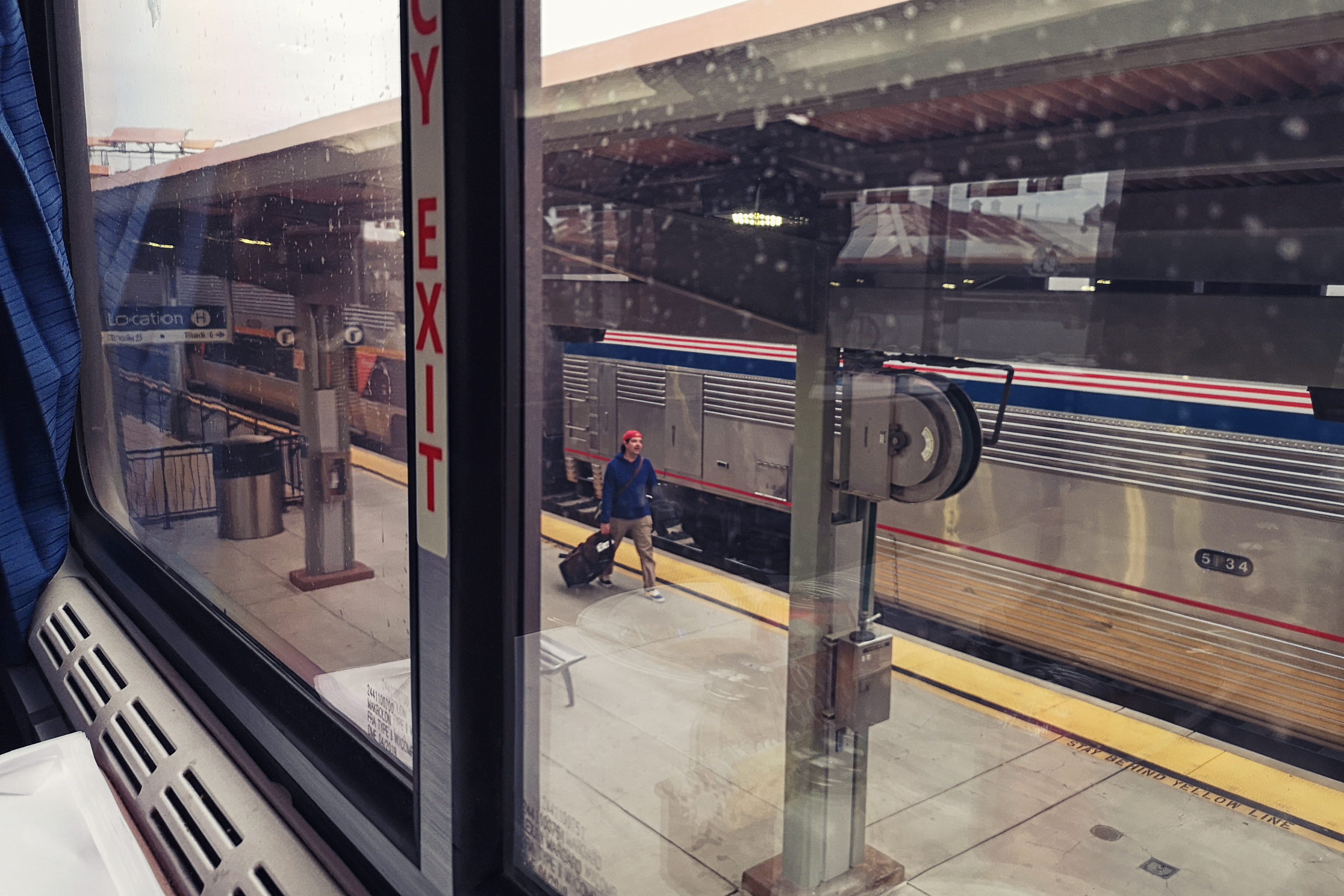
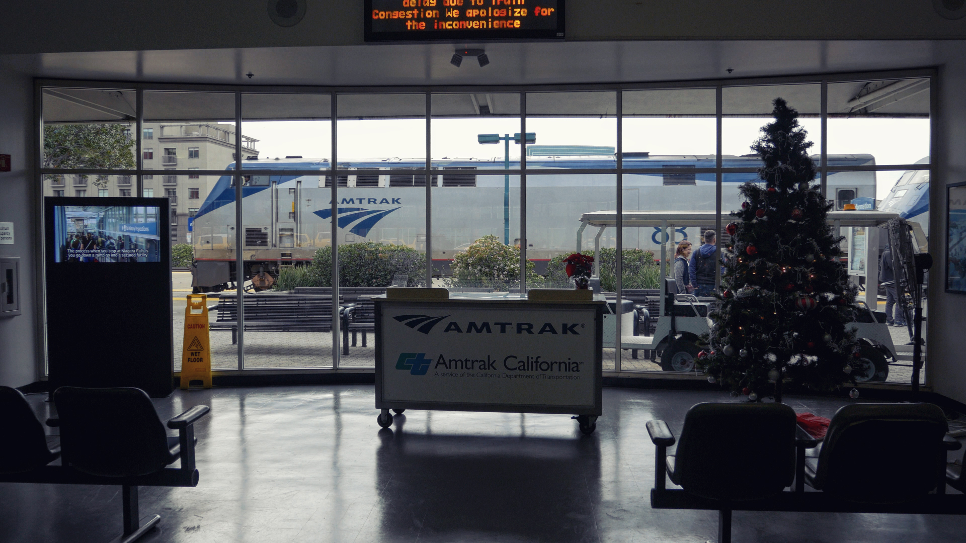
当地时间下午三点半左右,列车到达了终点站,旧金山郊外的爱莫利维尔(Emeryville),出乎意料的比预定时间早了四十分钟,可见列车的排图还是非常松的。
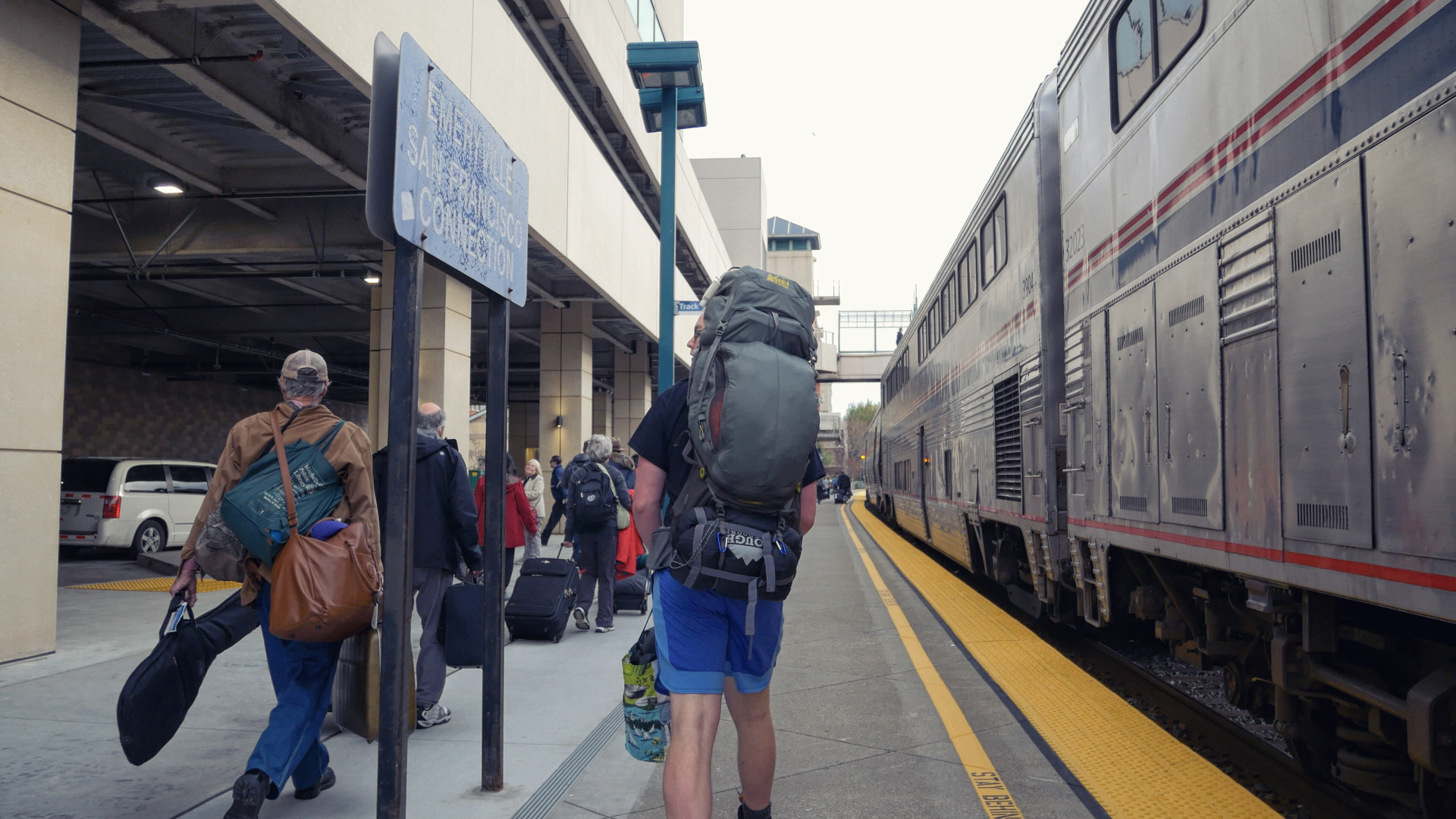 到达终点站
到达终点站
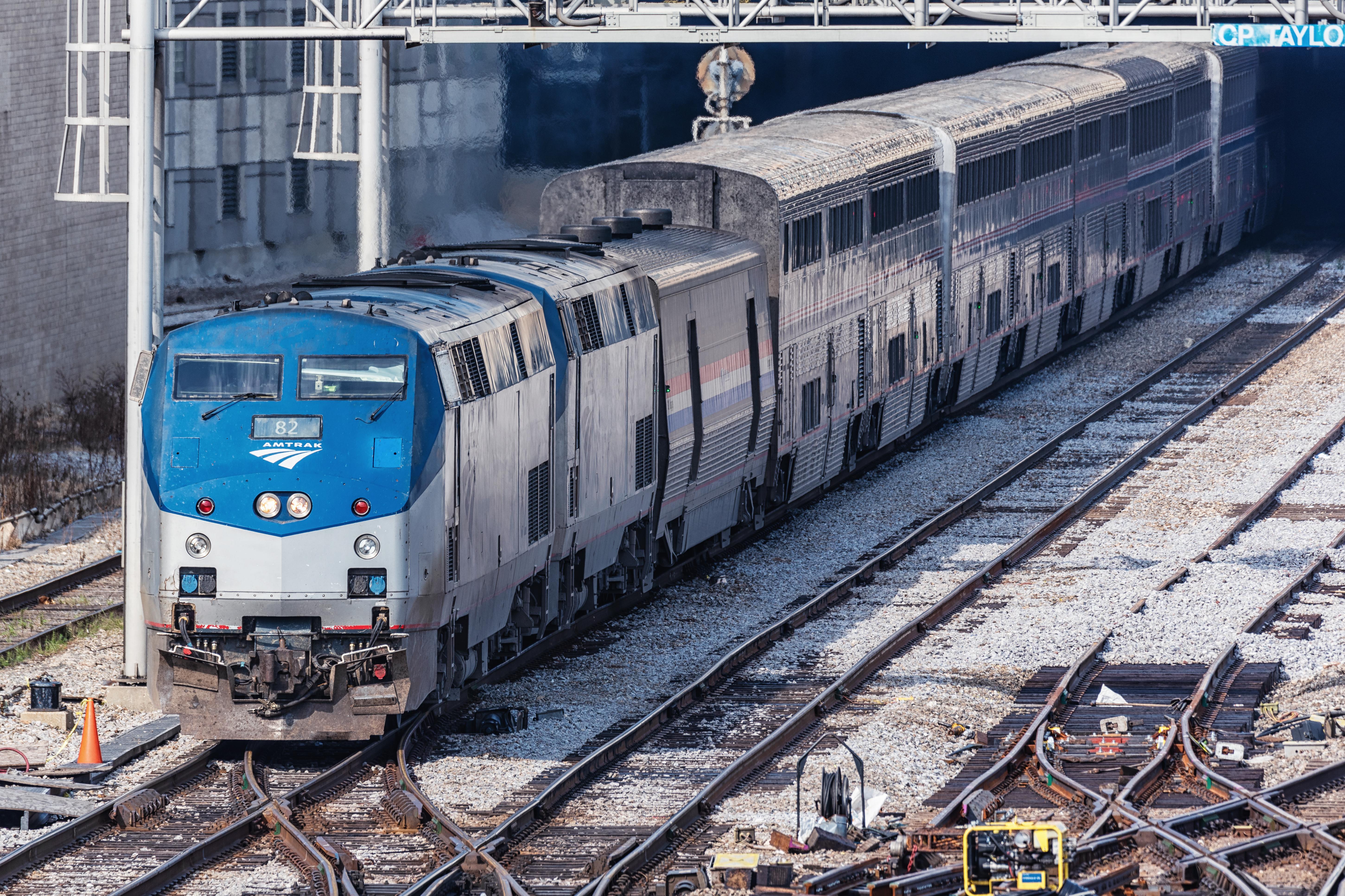
走到车头,看一看陪伴了我们三天两夜的列车,两台P42DC机车饱经风霜。
 停靠在站台的加州和风号
走进候车室,看着回送列车渐渐远去,52小时横穿美国的旅程也终于圆满的画上了句点。
 列车远去
列车远去
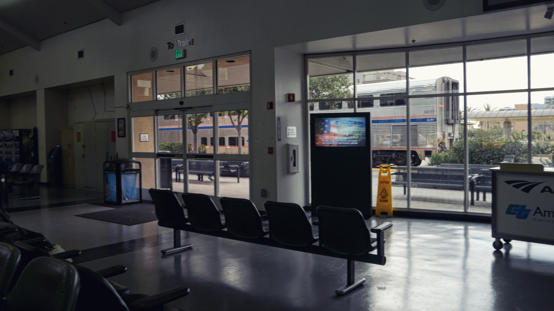 列车远去
列车远去
在候车室驻足良久,三天来的一切还历历在目。看到的雪山,沙漠,遇到的人,听到的故事,都将随着这趟旅程一起,成为生命中难以忘怀的一部分。
候车室外,人来人往,远处闪烁着城市繁华的灯火。我们踏上前往市区的巴士。加州和风号,望有朝一日能够再见!而新的旅程,刚刚开始!
一些攻略和补充
i. 关于买票。笔者是在Amtrak的官方app上购买的,购买后会收到电子票,打印出来去车站出示即可。电子票如下。
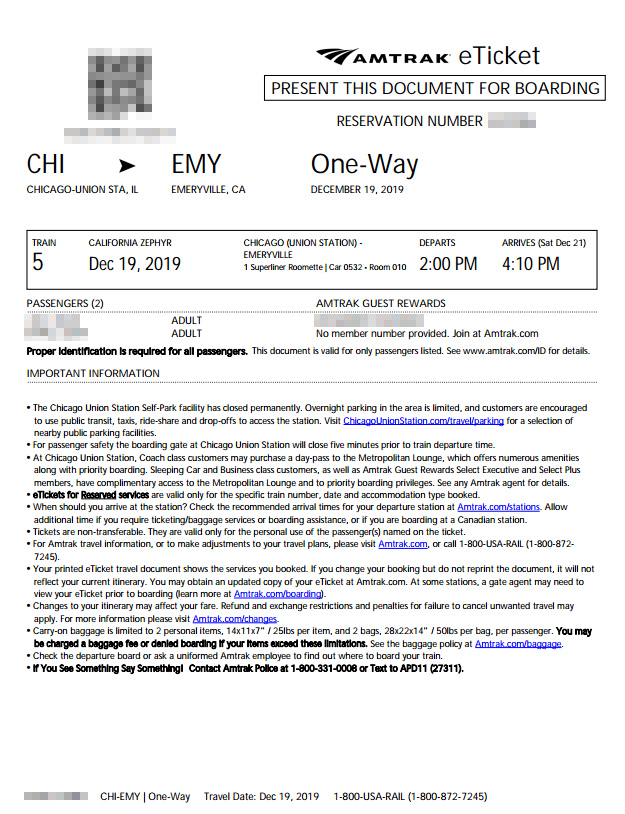 电子票
电子票
也可以去美铁的官网购买。然后之前提过,有些时候票可能会比较紧张,注意提前购买。票价的话是会浮动的。我们那时候只剩一张票并且赶上圣诞节前,所以票价比较高,两人1118刀含税。笔者查了下离现在大概一个月的2月14日的全程票价供大家参考。像我们这样的狭小二人间771刀,带厕所的宽广二人间2161刀,家庭套房1837刀。坐席最便宜的282刀(不可退款),最贵678刀(可取消并退款)。相对而言坐席会便宜很多。据说在晚上会有很多空座,可以座代卧,不过毕竟两夜,还是不太推荐尝试。
ii. 请准备一些现金,方便给小费。吃饭的时候和最后下车的时候按情理要给列车员小费。
iii. 车上没有WiFi,旅途中很多地方也是收不到手机信号的。可能年轻人不太能够接受这种生活,乘车的大多数是中老年人。然后也请尽量不要将需要网络的重要工作留到列车上做,毕竟随时可能断网。如果不是很能耐得住没有网络的寂寞的话,请提前准备好合适的娱乐方式。
iv. 之前也讲到过每个房间只有一个插座,可以考虑准备插线板。同时也可以询问列车员附近有没有可以用来充电的空房间。
v. 由于线路质量等等原因,车总体是比较晃的,在车内行走请注意安全,特别是通过车厢连接处的时候。
vi. 在终点站下车之后可以乘坐美铁的巴士去旧金山市中心,不用再换乘其他公共交通了。购买巴士票时出示火车票可以有折扣。
vii. 非常抱歉这次没有进入到坐席车内去拍照,如果需要了解坐席相关的情况可以去下面的美铁官网链接。
viii. 希望我的这篇文章能够或多或少的将旅行的风景展现给大家,也能给大家的出行带来一些帮助。非常感谢大家一路阅读到了这里,非常抱歉占用了大家的时间。如果有什么问题的话欢迎在评论里或者私信来询问,笔者会尽力回答。文章中的错误也非常欢迎指出。
一些链接
参考资料
[1] https://en.wikipedia.org/wiki/California_Zephyr
[2] https://www.amtrak.com/california-zephyr-train
Glovebox Pressure Control System for Redox Flow Battery
This is the capstone design project I conducted for the course ME 450 at the University of Michigan. My collaborators on this project are Tiantian Li, Junjie Luo, and Haoze Hu.
Goal
The goal of project “Glovebox Pressure Control System for Redox Flow Battery” is to develop a pressure sensing and control system that will maintain the pressure of a glovebox between variable set limits with automated gas inlet/exit valves. This system is intended to help the Kwabi lab at the University of Michigan create a platform for the testing of novel chemistries for redox-flow batteries that are sensitive to atmosphere.
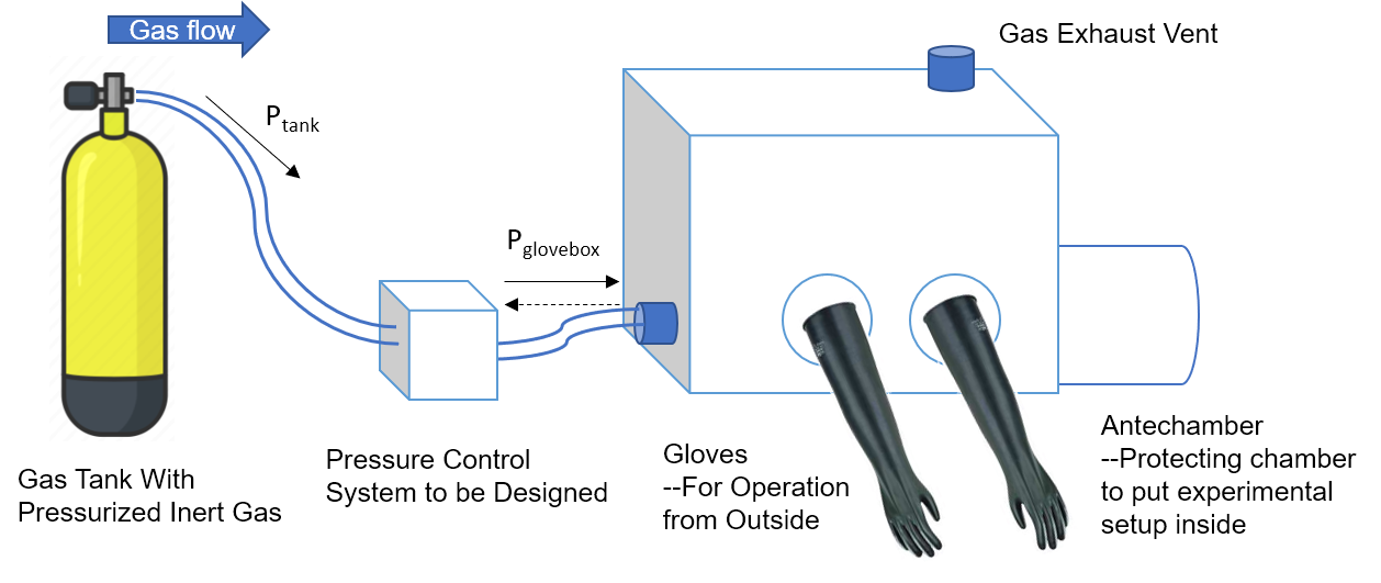 Schematic of the glovebox with key components labeled.
Requirements & Engineering Specifications
Relevant information was collected from various sources including literature review, benchmarking products and interviews with researchers from the Kwabi lab. The requirements and engineering specifications of the pressure sensing and control system are thus extrapolated and can be categorized into operation, safety and user related requirements. Key challenges of this project lie in the high-accuracy and high-resolution (±0.1 mbar) sensing and regulating of pressure in a low range of 0 – 20 mbar.
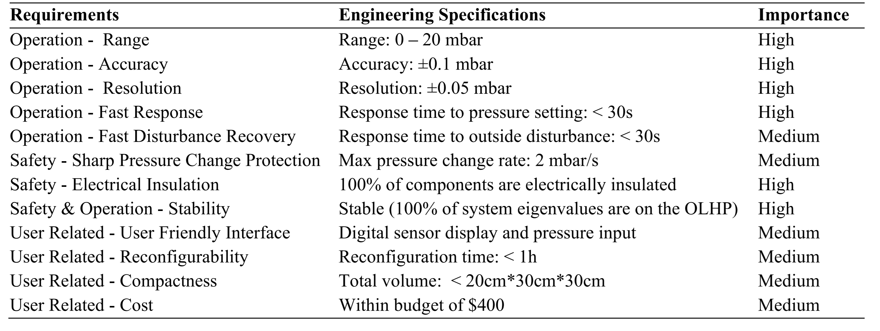 The requirements and their corresponding importance as well as engineering specification associated with the glove box pressure control system.
Concept Generation
Concepts generation process used two major methods, concept map and physical decomposition. Concept map helped incorporate broad aspects around the pressure control goal. Influencing aspects are connected and different traits of aspects are distinguished with colors. One important part of the concept map is the actuation methods to control the pressure. From the ideal gas law, pressure control can be changed with the amount of gas, volume and temperature. From these three directions, three concepts are developed. Physical decomposition helped break the complex systems into separate subsystems, including sensor, control, power and actuation. Actuation system are decomposed for each concept. These concepts are then evaluated with a Pugh chart, and the method to control the inflow and outflow of the gas with electronic valves are selected as the final solution with its high feasibility and potentially low cost.
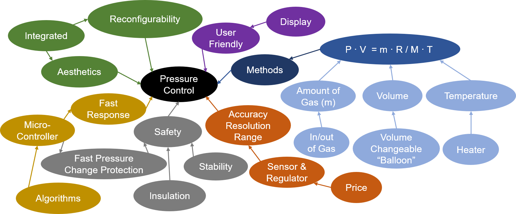 Concept map of the pressure control system. Different influential aspects are distinguished with colors, and the methods leads to three directions of concepts.
 Physical decomposition of the system that controls the inflow and outflow of gas with electrical valves.
Final Design
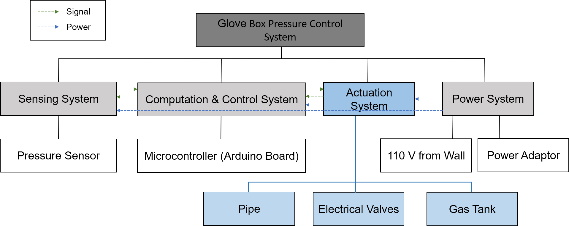
Our final design uses electric valves (flow coefficients Cv = 0.08 & 0.6) to control the gas in flow and out flow, and an on-off feedback control algorithm was performed using a pressure sensor and the Arduino board. Through engineering analysis, formula was generated to simulate the system behavior, which were used to select the flow coefficients of the electric valves and verify the engineering specifications.
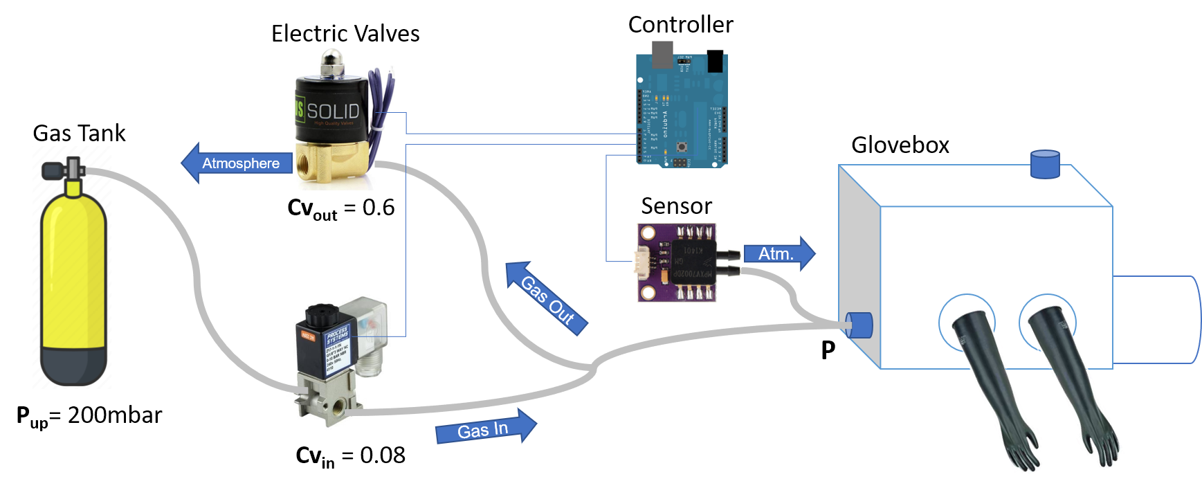 Illustration of the components of the final design solution.
General Validation Process
A full validation plan was developed for physical prototypes, and key specifications were validated virtually through performance simulation, including the disturbance rejection induced from glove movement volume change.
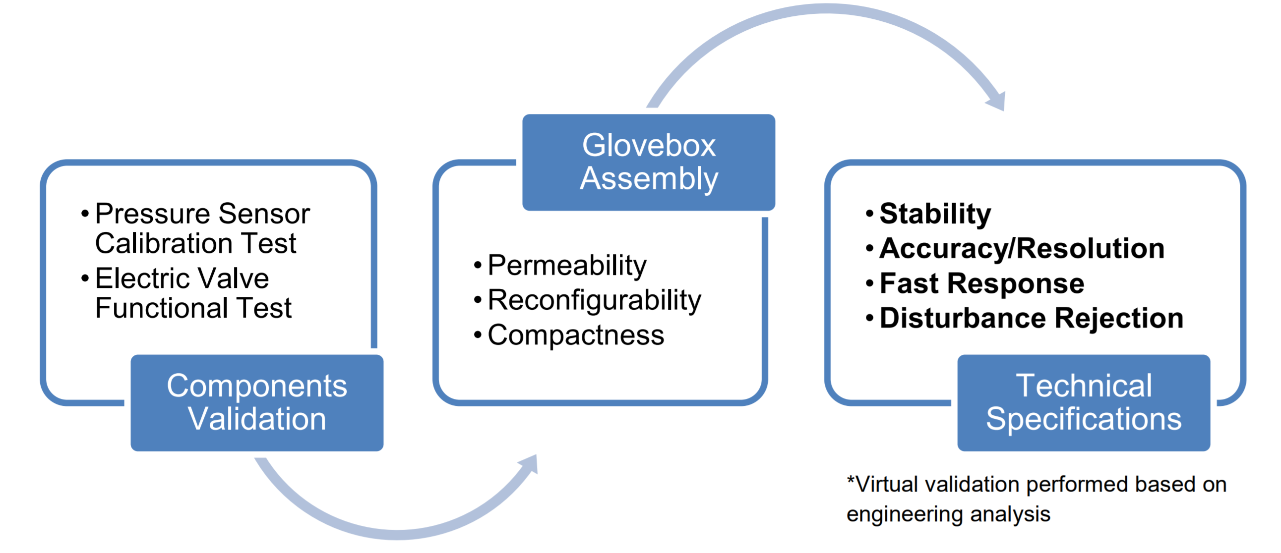 Validation Process Chart. Pressure controlling components are first validated with their functions and then assembled to the glovebox to verify the specifications and validate its functions.
Performance (by simulation)
The system was able to meet the specifications under reasonably slow glove movements.
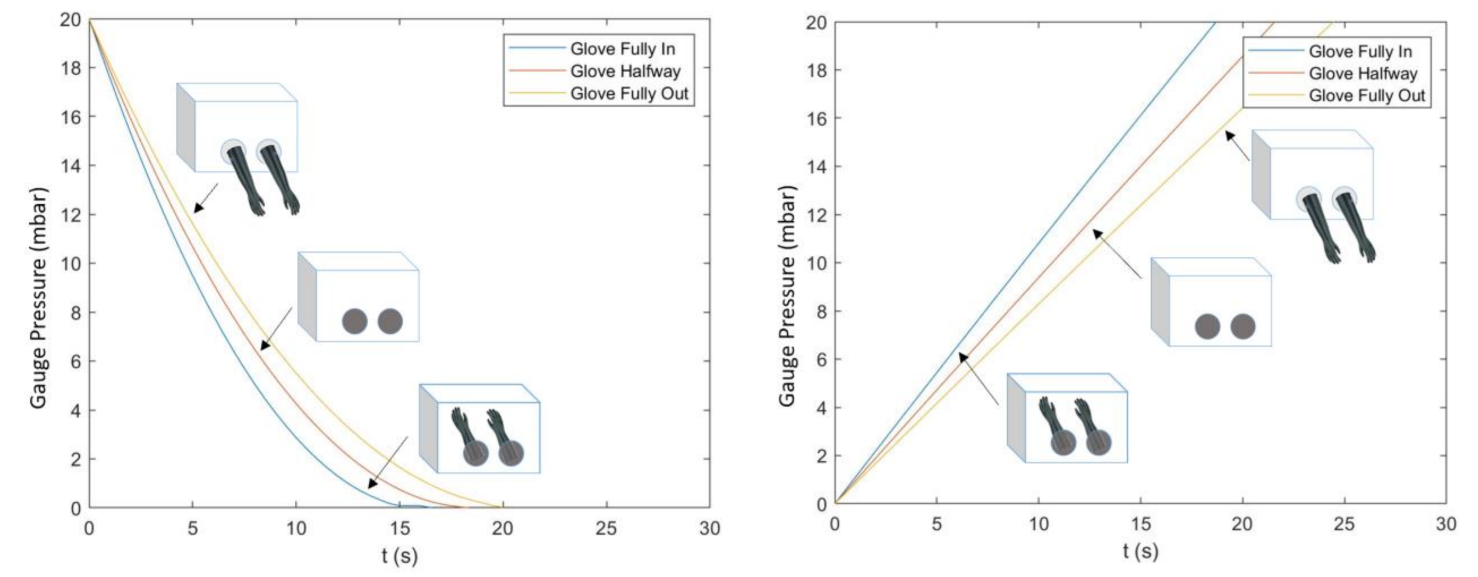 Simulation of maximum possible pressure change (20 mbar) for both the gas inflow (left) and outflow (right) cases at different glove box volumes. The simulation results show that the pressure changes more quickly at smaller volumes.
Future Improvements
In order to achieve faster glove movements, necessary improvements may be made to the system. There are two potential methods to solve this problem. The first method is to use an electric valve with changeable Cv value. When the difference between the current pressure and the desired pressure is big, the electric valve will work at high Cv value. As the current pressure is approaching the desired value, Cv value will be correspondingly decreasing to less than 0.1 for stability and accuracy. Accordingly, the program should be improved to control Cv value in real time based on the difference between the current pressure and the desired pressure. Although the electric valve with changeable Cv value works better, it costs much more.
If budget is limited, the second method can be considered: adding a pump to the pressure control system. The purpose of the pump is similar to what is discussed in the first method. When the difference between the current pressure and the desired pressure is large, the pump will be turned on to accelerate gas absorption/exhaustion. When the current pressure is close to the desired pressure, the pump will be shut down for stability and accuracy. Also, the program should be improved to control the pump in real time based on the difference between the current pressure and the desired pressure. In this case, the pump’s delay time should also be considered in the program. Compared with the former one, this method is cheaper, but the circuit will be more complex, and more parameters are introduced to the system (the pump’s delay time).
Conclusions
In general, this project achieves the pressure control function available in advanced and expensive glovebox workstations, which is built upon regular glovebox containers with a relatively low cost. It is a useful solution for the labs who need pressure-controlled testing environment but have restricted budgets.
Acknowledgements
We want to express our great appreciation to all those who contributed to the success of this project, including the team 09 members, our classmates in Section 05 who offered us useful suggestions, Heather and other Professors of ME 450 who taught us valuable knowledge and supported us, Professor Kaviany who met with us weekly to guide and help us, as well as Professor Kwabi and Mr. Modak who offered us this opportunity to work on the project and provided us with wonderful advises and questions along the way. Thank you very much for your help and it has been a pleasure working with you.
Arizona, USA, 2020 Winter Break Trip
During the winter break between Dec. 2019 and Jan. 2020, I went on a great trip across the US: starting from Michigan, I went to Illinois, took a train (the California Zephyr) to California, then drove to Nevada, Utah, and in the end Arizona. This trip took us 18 days and we found great joy in it, especially in photography.
We spent a total of 6 days in Arizona, including 1 day at Page, 3 days at the Grand Canyon, and 2 days at Phoenix. I have only posted the photos at the Grand Canyon for now. I will update the others in the future.
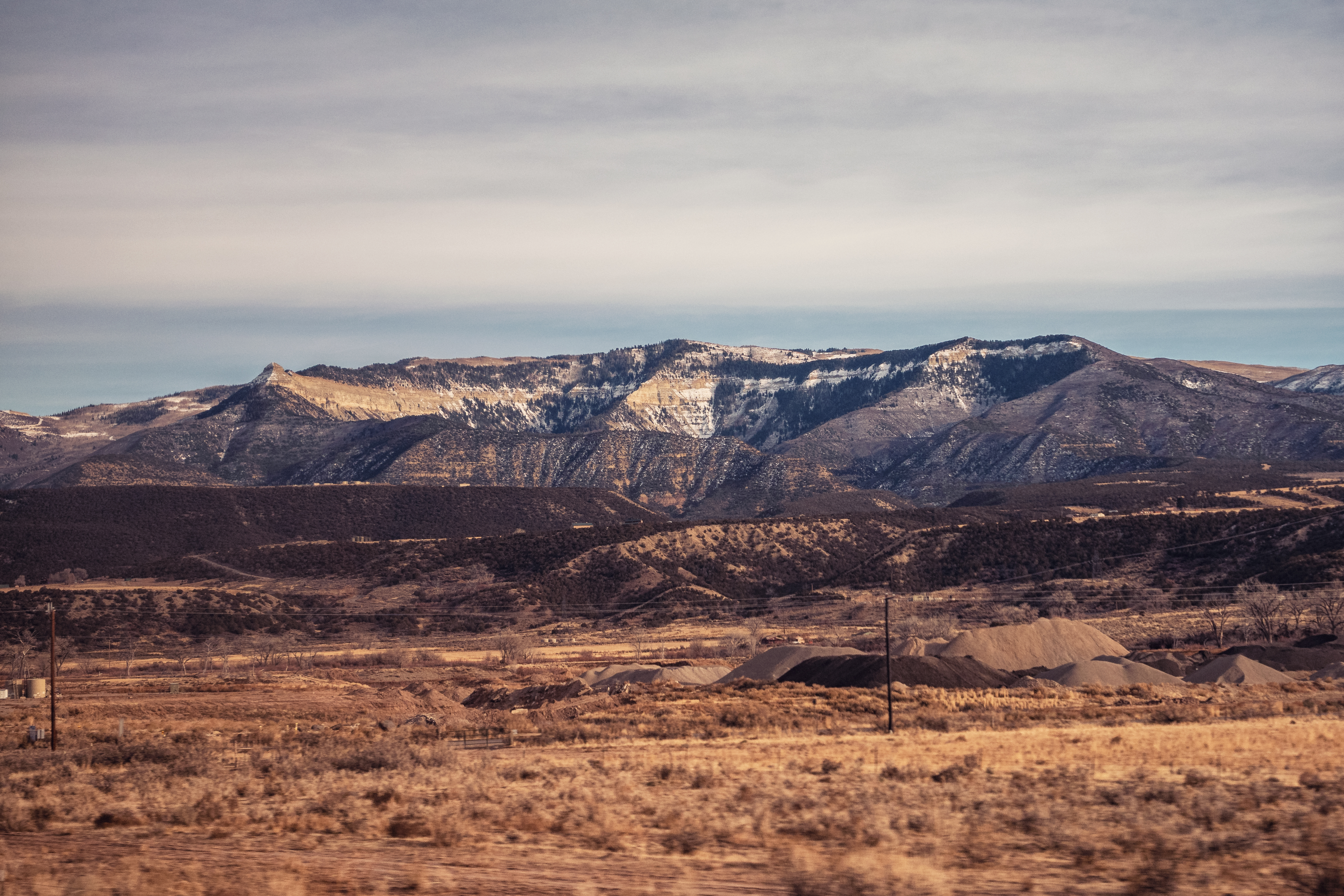
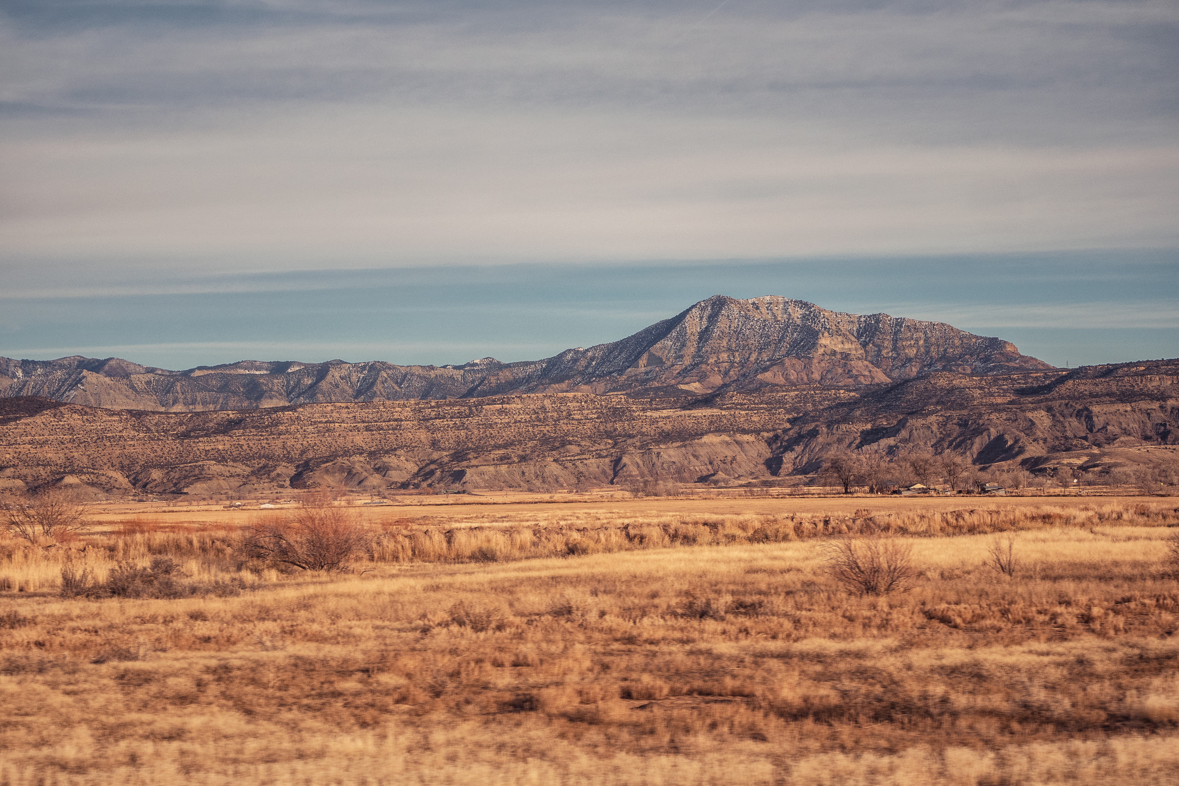
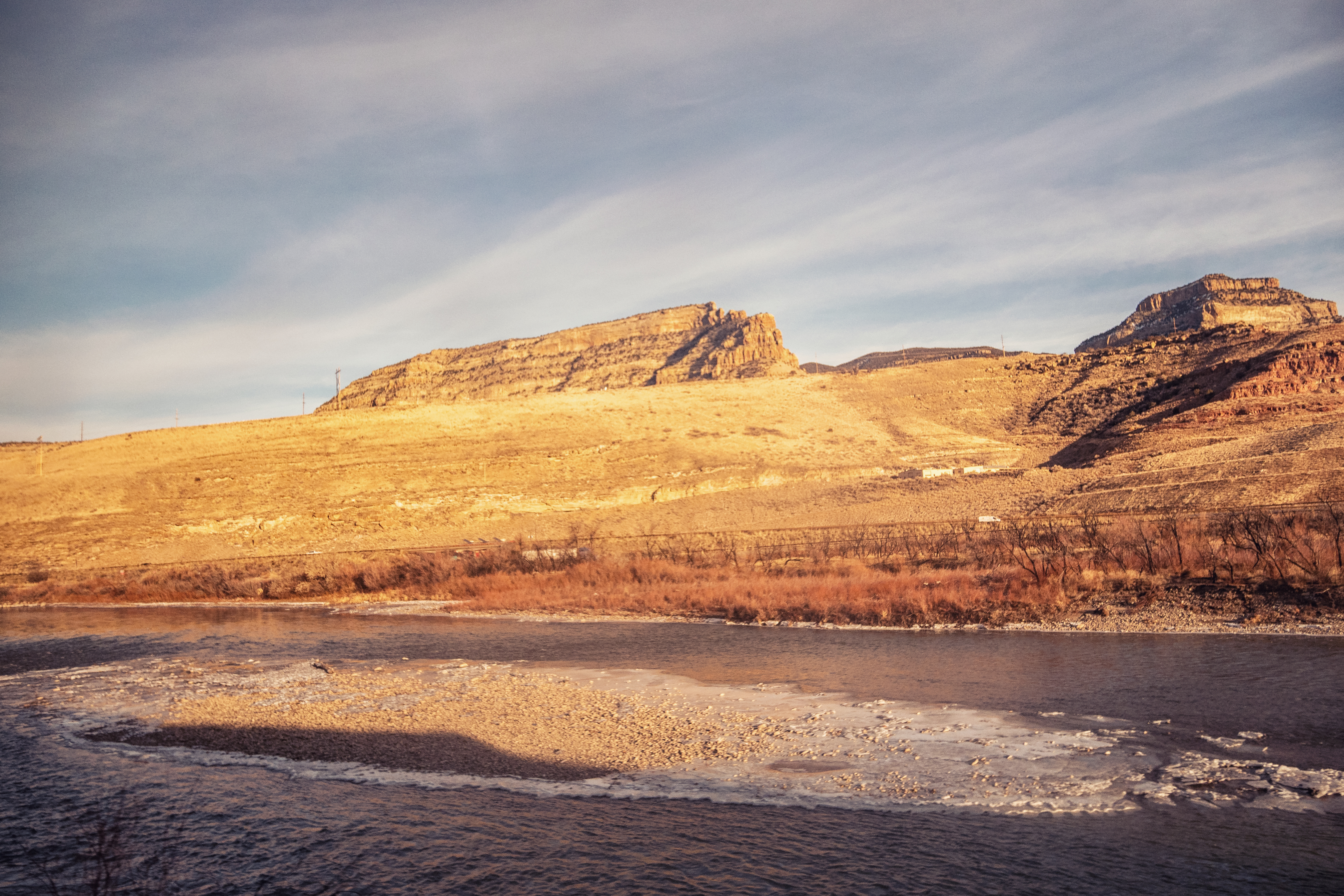
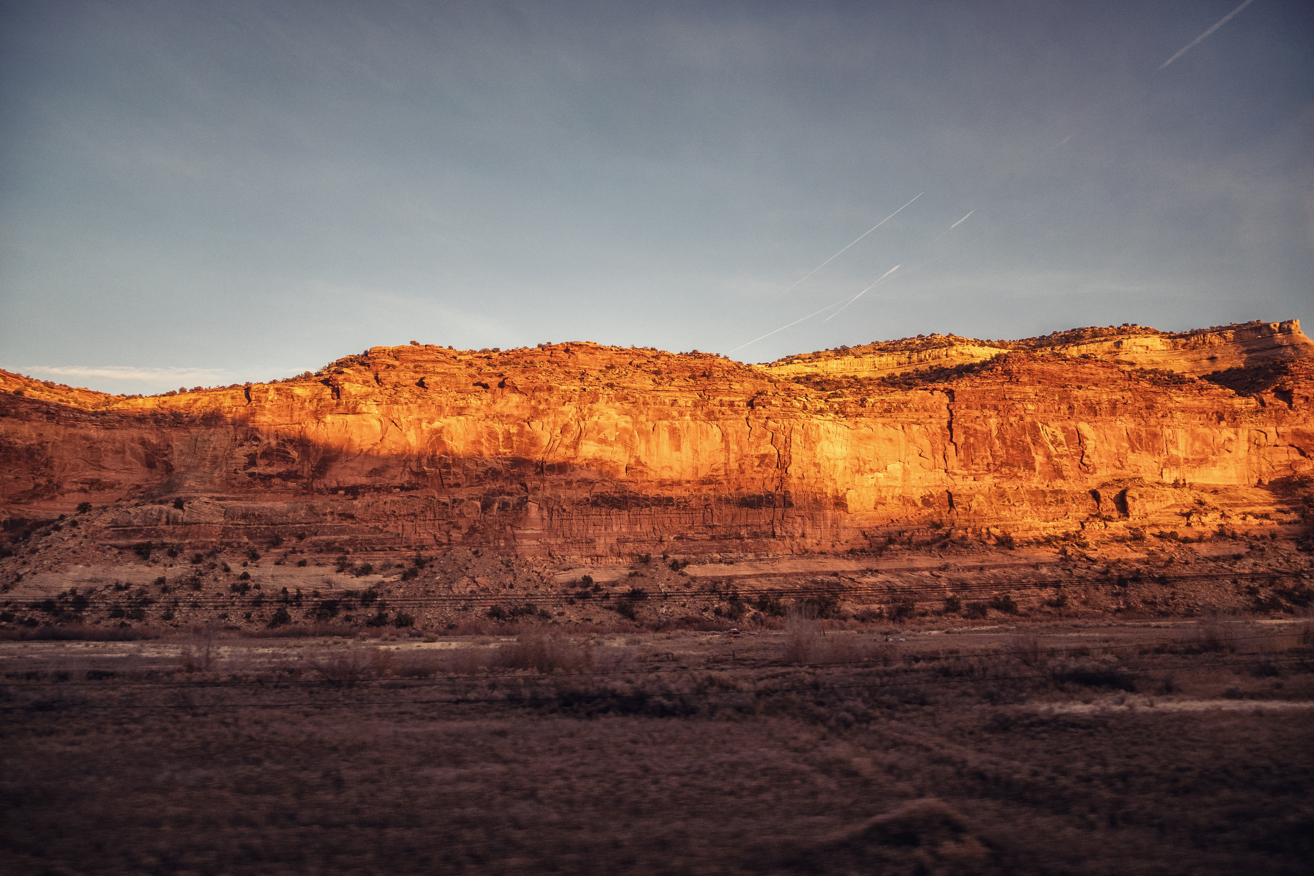
Utah, USA, 2020 Winter Break Trip
During the winter break between Dec. 2019 and Jan. 2020, I went on a great trip across the US: starting from Michigan, I went to Illinois, took a train (the California Zephyr) to California, then drove to Nevada, Utah, and in the end Arizona. This trip took us 18 days and we found great joy in it, especially in photography.
We spent a total of 2 days in Utah, most of which were spent on in the Monument Valley. It is one of the locations where the film “Forest Gump” was shot. The geology there was unique and beautiful: definitely a meaningful place to visit for a trip.
Nevada, USA, 2020 Winter Break Trip
During the winter break between Dec. 2019 and Jan. 2020, I went on a great trip across the US: starting from Michigan, I went to Illinois, took a train (the California Zephyr) to California, then drove to Nevada, Utah, and in the end Arizona. This trip took us 18 days and we found great joy in it, especially in photography.
We spent a total of 2 days in Nevada, most of which were spent on gambling and watching shows… It was a fantastic experience but in return there were few photos to share with you. Therefore, I put photo taken at the Death Valley (at the borderline of California and Nevada) here.